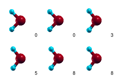
So far, we have calculated the energy of a water molecule with specified atom positions. This tutorial shows you how to optimize the geometry of the molecule (i.e. atom positions), and also how to continue a calculation.
This time, let's start with a very coarse geometry. In reality, the water molecule has an O-H bond length of roughly 0.97 Angstrom and a bond angle of 104.5 degrees. To give the geometry optimizer something to do, let's start with a bond length of 1 Angstrom and bond angle of 90 degrees. Save the following to water.xyz:
3

O  0.00  0.00  0.00
H  0.00  0.71  0.71
H  0.00 -0.71  0.71
Generate water.ionpos and water.lattice as in the previous tutorial using xyzToIonposOpt with a padding of 15 bohrs.
Next save the following water.in including ionic optimization:
include water.lattice
include water.ionpos
coords-type cartesian

coulomb-interaction Isolated
coulomb-truncation-embed 0 0 0

ion-species GBRV/$ID_pbe.uspp
elec-cutoff 20 100

dump-name water.$VAR    #Filename pattern for saving outputs
dump End State          #Output State i.e. everything needed to resume the calculation

ionic-minimize \
    nIterations 3 \
    energyDiffThreshold 1e-6 \
    knormThreshold 1e-4  #Threshold on RMS cartesian force
and run
jdftx -i water.in | tee water.out
Notice that in this run, after finishing one electronic minimize (lines starting with ElecMinimize), the calculation prints a line IonicMinimize with the same energy as the last prceding ElecMinimize step. The next entry on that line labelled |grad_K| is the RMS Cartesian force on the atoms. This line was present even in previous calculations without geometry optimization, but those calculations wrapped up after printing this line. This time, however, since the RMS force is larger than the threshold we specified, the IonicMinimize proceeds to update the atom positions and rerun ElecMinimize.
We can examine the progress of the ionic minimizer by pulling out the lines containing IonicMinimize:
grep IonicMinimize water.out
Note that the geometry optimizer updates the ionic positions three times (limited by the nIterations we specified), but does not yet reach the RMS force or energy-difference convergence criteria we specified. Fortunately, we asked the calculation to output its state. In this case it output water.wfns containing the converged wavefunctions and also updated the geometry in water.ionpos (grep Dumping water.out).
To continue the calculation, add the initial-state command to water.in:
initial-state water.$VAR #Filename pattern to search for initial state
update nIterations in IonicMinimize to 10 (I chose 3, which is too small, specifically to demonstrate continuation), and rerun jdftx
jdftx -i water.in | tee -a water.out #The -a says append to water.out
Examine the output file again. (If you appended the outut file as indicated above, scroll past the first calculation to where the second one begins.) Note that unlike previous times, the calculation skips the LCAOMinimize section because the wavefunctions have already been read in. The first ElecMinimize completes very quickly since it starts with previously converged wavefunctions at the last ionic positions. Look at the remaining ionic steps (using grep IonicMinimize again): the geometry optimizer now converges with RMS forces within the threshold we specified.
Calculate the DFT-predicted bond length and angle from the final water.ionpos. With the GBRV pseudopotentials and the PBE exchange-correlation functional, I get a converged O-H bond length of 0.98 A and an H-O-H bond angle of 103.7 degrees.
We can visualize the geometry optimization steps using:
createXSF water.out water.axsf Animated
Unfortunately, VESTA, that we have been using so far (and that has a more polished interface), does not support animated XSF files. Open this file in XCrysDen instead, and you should be able to click through a number of slides corresponding to the geometry optimization steps. As before, you need to change the boundary settings to see the molecule intact instead of torn across the boundaries. Change the unit of repetition in the XCrysDen menu: Display -> Unit of Repetition -> Translational asymmetric unit.