We have so far calculated the phonon dispersion relation from the force matrix using code very similar to the Wannier interpolation of the electronic band structure. We can combined these techniques along with Wannier interpolation of electron-phonon matrix elements to efficiently calculate properties related to electron-phonon coupling, such as the Eliashberg spectral function and the resistivity of metals.

First, let us expand on the Aluminum calculation from the Entangled bands tutorial to add phonon-related properties:

#Save the following to phonon.in
include totalE.in
initial-state totalE.$VAR
dump-only

phonon supercell 2 2 2

which can be run with "mpirun -n 4 phonon -i phonon.in | tee phonon.out". For a quick test, we have used a small phonon supercell that can be run in about a minute on a laptop. Realistic calculations should use larger phonon supercells, typically at least 4x4x4.

The phonon calculation produces a 'totalE.phononHsub' file containing electron-phonon matrix elements in a atom-displacement - Bloch function basis, which we have not used so far. We need to convert these matrix elements to a atom displacement - Wannier basis in order to interpolate to electron-phonon matrix elements at arbitrary wave vectors. We need to rerun wannier with an additional parameter so that it performs this conversion:

#Edit the wannier command in wannier.in so that it becomes:
wannier \
    innerWindow -0.042 0.693 \
    outerWindow -0.042 1.024 \
    saveMomenta yes \
    phononSupercell 2 2 2  #this should match the supercell in phonon.in

After updating wannier.in, rerun "mpirun -n 4 wannier -i wannier.in | tee wannier.out" which will produce the electron-phonon matrix elements in wannier.mlwfHePh, along with the corresponding cell maps etc.

In order to use these matrix elements, we need to perform a double Fourier transform, followed by unitary rotations to bring to the eigen-basis of both electronic states and the phonon state involved:

\[ g^{\vec{q}\beta}_{\vec{k}b,\vec{k}'b'} = \frac{1}{\sqrt{2\omega^{\mathrm{ph}}_{\vec{q}\beta}}} \sum_{\alpha} U^{\mathrm{(ph)}\vec{q}}_{\alpha\beta} \sum_{\vec{R}\vec{R}'aa'} e^{i\vec{k}'\cdot\vec{R}'-i\vec{k}\cdot\vec{R}} \left( U^{\vec{k}\dagger}_{ba} \tilde{g}^{\beta}_{\vec{R}a,\vec{R}'a'} U^{\vec{k}'}_{a'b'} \right)$$ \]

This logic is implemented within the calcEph() function of the python script shown below. This script used the interpolated electron-phonon matrix elements to compute the transport-weighted Eliashberg spectral function:

\[ \alpha_v^2F(\omega) = \frac{g_s^2}{N_{\vec{k}}N_{\vec{k}'}g(\mu)^2} \sum_{\vec{k}\vec{k}'bb'\alpha} \delta(\omega-\omega_{\vec{q}\alpha}) \delta(\varepsilon_{\vec{k}b}-\mu)\delta(\varepsilon_{\vec{k}'b'}-\mu) \left| g^{\vec{k}'-\vec{k},\alpha}_{\vec{k}'b',\vec{k}b} \right|^2 \left(1 - \frac{\vec{v}_{\vec{k}b}\cdot\vec{v}_{\vec{k}'b'}}{|\vec{v}_{\vec{k}b}| |\vec{v}_{\vec{k}'b'}|}\right). \]

and using that, computes the conductivity (as a function of temperature) as:

\[ \sigma = \frac{e^2v_F^2}{3} \left[ \frac{2\pi}{\hbar} \int d\omega \alpha_v^2F(\omega) \frac{\frac{\hbar\omega}{k_BT}\exp\frac{\hbar\omega}{k_BT}} {\left(\exp\frac{\hbar\omega}{k_BT}-1\right)^2} \right]^{-1} \]

The following script computes the Eliashberg spectral function and resistivity as discussed above:

#Save the following to WannierEph.py:
import matplotlib.pyplot as plt
import numpy as np
import sys

#Read the MLWF cell map, weights and Hamiltonian:    
cellMap = np.loadtxt("wannier.mlwfCellMap")[:,0:3].astype(np.int)
Wwannier = np.fromfile("wannier.mlwfCellWeights")
nCells = cellMap.shape[0]
nBands = int(np.sqrt(Wwannier.shape[0] / nCells))
Wwannier = Wwannier.reshape((nCells,nBands,nBands)).swapaxes(1,2)
#--- Get k-point folding from totalE.out:
for line in open('totalE.out'):
    if line.startswith('kpoint-folding'):
        kfold = np.array([int(tok) for tok in line.split()[1:4]])
kfoldProd = np.prod(kfold)
kStride = np.array([kfold[1]*kfold[2], kfold[2], 1])
#--- Read reduced Wannier Hamiltonian, momenta and expand them:
Hreduced = np.fromfile("wannier.mlwfH").reshape((kfoldProd,nBands,nBands)).swapaxes(1,2)
Preduced = np.fromfile("wannier.mlwfP").reshape((kfoldProd,3,nBands,nBands)).swapaxes(2,3)
iReduced = np.dot(np.mod(cellMap, kfold[None,:]), kStride)
Hwannier = Wwannier * Hreduced[iReduced]
Pwannier = Wwannier[:,None] * Preduced[iReduced]

#Read phonon dispersion relation:
cellMapPh = np.loadtxt('totalE.phononCellMap', usecols=[0,1,2]).astype(int)
nCellsPh = cellMapPh.shape[0]
omegaSqR = np.fromfile('totalE.phononOmegaSq') #just a list of numbers
nModes = int(np.sqrt(omegaSqR.shape[0] // nCellsPh))
omegaSqR = omegaSqR.reshape((nCellsPh, nModes, nModes)).swapaxes(1,2)

#Read e-ph matrix elements
cellMapEph = np.loadtxt('wannier.mlwfCellMapPh', usecols=[0,1,2]).astype(int)
nCellsEph = cellMapEph.shape[0]
#--- Get phonon supercell from phonon.out:
for line in open('phonon.out'):
    tokens = line.split()
    if len(tokens)==5:
        if tokens[0]=='supercell' and tokens[4]=='\\':
            phononSup = np.array([int(token) for token in tokens[1:4]])
prodPhononSup = np.prod(phononSup)
phononSupStride = np.array([phononSup[1]*phononSup[2], phononSup[2], 1])
#--- Read e-ph cell weights:
nAtoms = nModes // 3
cellWeightsEph = np.fromfile("wannier.mlwfCellWeightsPh").reshape((nCellsEph,nBands,nAtoms)).swapaxes(1,2)
cellWeightsEph = np.repeat(cellWeightsEph.reshape((nCellsEph,nAtoms,1,nBands)), 3, axis=2) #repeat atom weights for 3 directions
cellWeightsEph = cellWeightsEph.reshape((nCellsEph,nModes,nBands)) #coombine nAtoms x 3 into single dimension: nModes
#--- Read, reshape and expand e-ph matrix elements:
iReducedEph = np.dot(np.mod(cellMapEph, phononSup[None,:]), phononSupStride)
HePhReduced = np.fromfile('wannier.mlwfHePh').reshape((prodPhononSup,prodPhononSup,nModes,nBands,nBands)).swapaxes(3,4)
HePhWannier = cellWeightsEph[:,None,:,:,None] * cellWeightsEph[None,:,:,None,:] * HePhReduced[iReducedEph][:,iReducedEph]

#Constants / calculation parameters:
mu = 0.399     #in Hartrees
eV = 1/27.2114 #in Hartrees
omegaMax = 6*eV #maximum photon energy to consider
Angstrom = 1/0.5291772 #in bohrs
aCubic = 4.05*Angstrom #in bohrs
Omega = (aCubic**3)/4  #cell volume

#Calculate energies, eigenvectors and velocities for given k
def calcE(k):
    #Fourier transform to k:
    phase = np.exp((2j*np.pi)*np.dot(k,cellMap.T))
    H = np.tensordot(phase, Hwannier, axes=1)
    P = np.tensordot(phase, Pwannier,  axes=1)
    #Diagonalize and switch to eigen-basis:
    E,U = np.linalg.eigh(H) #Diagonalize
    v = np.imag(np.einsum('kba,kibc,kca->kai', U.conj(), P, U)) #diagonal only
    return E, U, v

#Calculate phonon energies and eigenvectors for given q
def calcPh(q):
    phase = np.exp((2j*np.pi)*np.tensordot(q,cellMapPh.T, axes=1))
    omegaSq, U = np.linalg.eigh(np.tensordot(phase, omegaSqR, axes=1))
    omegaPh = np.sqrt(np.maximum(omegaSq, 0.))
    return omegaPh, U

#Calculate e-ph matrix elements, along with ph and e energies, and e velocities
def calcEph(k1, k2):
    #Electrons:
    E1, U1, v1 = calcE(k1)
    E2, U2, v2 = calcE(k2)
    #Phonons for all pairs pf k1 - k2:
    omegaPh, Uph = calcPh(k1[:,None,:] - k2[None,:,:])
    #E-ph matrix elements for all pairs of k1 - k2:
    phase1 = np.exp((2j*np.pi)*np.dot(k1,cellMapEph.T))
    phase2 = np.exp((2j*np.pi)*np.dot(k2,cellMapEph.T))
    normFac = np.sqrt(0.5/np.maximum(omegaPh,1e-6))
    g = np.einsum('Kbd,kKycb->kKycd', U2, #Rotate to electron 2 eigenbasis
        np.einsum('kac,kKyab->kKycb', U1.conj(), #Rotate to electron 1 eigenbasis
        np.einsum('kKxy,kKxab->kKyab', Uph, #Rotate to phonon eigenbasis
        np.einsum('KR,kRxab->kKxab', phase2, #Fourier transform from r2 -> k2
        np.einsum('kr,rRxab->kRxab', phase1.conj(), #Fourier transform from r1 -> k1
        HePhWannier))))) * normFac[...,None,None] #Phonon amplitude factor
    return g, omegaPh, E1, E2, v1, v2

#Select points near Fermi surface on Brillouin zone:
Nk = 1000
Nblocks = 100
NkTot = Nk*Nblocks
#--- collect Fermi level DOS and velocities
dos0 = 0. #density of states at the fermi level
vFsq = 0. #average Fermi velocity
Esigma = 0.001 #Gaussian broadening of delta-function
kFermi = [] #k-points which contribute near the Fermi surface
print('Sampling Fermi surface:', end=' ')
for iBlock in range(Nblocks):
    kpoints = np.random.rand(Nk, 3)
    E,_,v = calcE(kpoints)
    #Calculate weight of each state being near Fermi level
    w = np.exp(-0.5*((E-mu)/Esigma)**2) * (1./(Esigma*np.sqrt(2*np.pi)))
    dos0 += np.sum(w)
    vFsq += np.sum(w * np.sum(v**2, axis=-1))
    #Select k-points that matter:
    sel = np.where(np.max(w, axis=1) > 1e-3/Esigma)[0]
    kFermi.append(kpoints[sel])
    print(iBlock+1, end=' '); sys.stdout.flush()
print()
vFsq *= 1./dos0 #now average velocity
dos0 *= (2./(Omega * NkTot))
kFermi = np.vstack(kFermi)
NkFermi = kFermi.shape[0]
print('vF:', np.sqrt(vFsq))
print('dos0:', dos0)
print('NkFermi:', NkFermi, 'of NkTot:', NkTot)

#Collect transport -weighted Eliashberg spectral function
blockSize = 64
Nblocks = 100
#--- phonon frequency grid
meV = 1e-3/27.2114
domegaPh = 0.1*meV
omegaPhBins = np.arange(0., 40.*meV, domegaPh)
omegaPhMid = 0.5*(omegaPhBins[:-1] + omegaPhBins[1:])
F = np.zeros(omegaPhMid.shape) #spectral function
print('Sampling transport spectral function:', end=' ')
for iBlock in range(Nblocks):
    #Select blocks of k-points from above set:
    k1 = kFermi[np.random.randint(NkFermi, size=blockSize)]
    k2 = kFermi[np.random.randint(NkFermi, size=blockSize)]
    #Get e-ph properties
    g, omegaPh, E1, E2, v1, v2 = calcEph(k1, k2)
    #Velocity direction factor:
    vHat1 = v1 * (1./np.linalg.norm(v1, axis=-1)[...,None])
    vHat2 = v2 * (1./np.linalg.norm(v2, axis=-1)[...,None])
    vFactor = 1. - np.einsum('kai,Kbi->kKab', vHat1, vHat2)
    #Term combining matrix elements and velocity factors, summed over bands:
    w1 = np.exp(-0.5*((E1-mu)/Esigma)**2) * (1./(Esigma*np.sqrt(2*np.pi)))
    w2 = np.exp(-0.5*((E2-mu)/Esigma)**2) * (1./(Esigma*np.sqrt(2*np.pi)))
    term = np.einsum('ka,Kb,kKab,kKxab->kKx', w1, w2, vFactor, np.abs(g)**2)
    #Histogram by phonon frequency:
    F += np.histogram(omegaPh.flatten(), omegaPhBins, weights=term.flatten())[0]
    print(iBlock+1, end=' '); sys.stdout.flush()
print()
F *= (4./(domegaPh * (NkTot*dos0)**2)) #factors from expression above
F *= (NkFermi**2)*1./(Nblocks*(blockSize**2)) #account for sub-sampling
#--- plot:
plt.figure(1, figsize=(5,3))
plt.plot(omegaPhMid/meV, F)
plt.ylabel(r'$\alpha^2 F(\omega)$ [a.u.]')
plt.xlabel(r'$\hbar\omega$ [meV]')
plt.xlim(0, 40.)
plt.ylim(0, None)
plt.savefig('SpectralFunction.png', bbox_inches='tight')

#Compute resistivity from spectral function:
Kelvin = 1./3.1577464e5 #in Hartrees
T = np.logspace(1,3)*Kelvin
betaOmega = omegaPhMid[:,None] / T[None,:] #hbar omega/kT
boseTerm = betaOmega*np.exp(betaOmega)/(np.exp(betaOmega)-1.)**2
Fint = domegaPh * np.dot(F, boseTerm)
rho = 2*np.pi*Fint/(Omega*vFsq/3) #in atomic units
#--- plot:
plt.figure(2, figsize=(5,3))
Ohm = 2.434135e-04
nm = 10/0.5291772
plt.loglog(T/Kelvin, rho/(Ohm*nm))
plt.scatter([300.], [26.5], marker='+', s=50) #Expt
plt.xlabel(r'$T$ [K]')
plt.ylabel(r'$\rho(T)$ [n$\Omega$m]')
plt.ylim(1e-2, 1e2)
plt.savefig('rhoVsT.png', bbox_inches='tight')
plt.show()

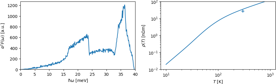
This script closely follows the structure of previous phonon and Wannier processing scripts. It reads the matrix elements and cell maps for electrons, phonons and the electron-phonon coupling. It then performs a Monte Carlo scan through the Brillouin zone to find k-points with states near the Fermi level, and then another Monte Carlo sampling through pairs of k-points to compute the transport-weighted Eliashberg spectral function. Running the script should produce these plots of the spectral function and resistivity versus temperature:

Note the modest agreement with the experimental resistivity of aluminum at room temperature, even with rather coarse sampling and a tiny 2x2x2 phonon supercell.

Exercise: repeat with a larger 4x4x4 phonon supercell using a compute cluster, and converge the above results with respect to Monte Carlo sampling of the Brillouin zone.