 |
JDFTx
1.7.0
|


|
|
JDFTx
1.7.0
|
|
In the previous tutorial, we calculated the total energy of silicon and explored its Brillouin zone convergence. This tutorial illustrates calculations of the electronic band structure, specifically, the variation of the Kohn-Sham eigenvalues along a special kpoint path in the Brillouin zone. It will also introduce an alternate algorithm for converging the electronic state, the self-consistent field (SCF) method.
First lets specify the common specifications for bulk silicon (same as previous tutorial):
#Save the following to common.in:
lattice face-centered Cubic 10.263
ion-species GBRV/$ID_pbe.uspp
elec-cutoff 20 100

ion Si 0.00 0.00 0.00  0
ion Si 0.25 0.25 0.25  0
and a total energy calculation:
#Save the following to totalE.in:
include common.in
kpoint-folding 8 8 8    #Use a Brillouin zone mesh
electronic-SCF          #Perform a Self-Consistent Field optimization
dump-name totalE.$VAR
dump End State BandEigs #State and band eigenvalues
dump End ElecDensity    #Save the self-consistent electron density
dump End EigStats       #Get eigenvalue statistics
which we run with
mpirun -n 4 jdftx -i totalE.in | tee totalE.out
Note the new command electronic-scf, which uses a different algorithm from the variational minimize to solve the Kohn-Sham equations. Essentially, Kohn-Sham eigenvalues and orbitals are calculated for an input potential, and a new density and potential are constructed from those orbitals. This output potential would in general be different from the input one, so the above step is repeated with successive guesses for the input potential until the input and output potentials become identical (within some threshold). In practice, the guess for the input potential at one step is based on input and output potentials from several previous steps (Pulay algorithm).
Examine the output file: instead of ElecMinimize lines, you will find lines starting with SCF, which report the change in energy and eigenvalues between "cycles". This algorithm is usually faster than the variational minimize, but unlike the default minimize algorithm, it is not guaranteed to converge.
Note that whether we used SCF or Minimize is not important for the remainder of this tutorial demonstrating band structure calculations; we will interchangeably use both algorithms for total energy calculations from now on to gain familiarity with both.
Next, we list high-symmetry points in the Brillouin zone laying out a path along which we want the band structure:
#Save the following to bandstruct.kpoints.in
kpoint 0.000 0.000 0.000     Gamma
kpoint 0.000 0.500 0.500     X
kpoint 0.250 0.750 0.500     W
kpoint 0.500 0.500 0.500     L
kpoint 0.000 0.000 0.000     Gamma
kpoint 0.375 0.750 0.375     K
For common crystal structures, you can find the high-symmetry points easily on the web, eg. this course website. For a more complete listing, you can consult a crystallography database eg. the Bilbao database, but to use that, you will first need to find the space group of your crystal.
From the above path specification, we can generate a sequence of points along the path and a plot script by running bandstructKpoints (in the jdftx/scripts directory):
bandstructKpoints bandstruct.kpoints.in 0.05 bandstruct
This should generate a file bandstruct.kpoints containing kpoints along the high-symmetry path and a GNUPLOT script bandstruct.plot. The second parameter, dk, of bandstructKpoints specifies the typical distance between kpoints in (dimensionless) reciprocal space; decreasing dk will produce more points along the path, which will take longer to calculate, but produce a smoother plot. Note that the last column of banstruct.kpoints.in is a label for the special Brillouin zone point which is used to label the plot.
Now we can run a band structure calculation along this path with the input file:
#Save the following to bandstruct.in
include common.in
include bandstruct.kpoints         #Get kpoints along high-symmetry path created above
fix-electron-density totalE.$VAR   #Fix the electron density (not self-consistent)
elec-n-bands 10                    #Number of bands to solve for
dump End BandEigs                  #Output the band eigenvalues for plotting
dump-name bandstruct.$VAR          #This prefix should match the final paramater given to bandstructKpoints
which we run using:
mpirun -n 4 jdftx -i bandstruct.in | tee bandstruct.out
which produces bandstruct.eigenvals. Finally running
gnuplot --persist bandstruct.plot
will generate a plot of the electronic band structure.
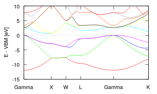
Note that the y-axis (energy) is in Hartrees and its absolute value is not particularly meaningful because the electrostatic potential in a 3D periodic system does not have an unambiguous zero reference point. Typically electronic band structure plots are referenced to the valence band maximum (VBM or HOMO) energy at zero for insulators, or the Fermi level for metals. Look at the eigStats output from the total energy calculation (totalE.eigStats) to identify the VBM (HOMO) energy and replace the final line of the auto-generated bandstruct.plot with the following lines:
set xzeroaxis               #Add dotted line at zero energy
set ylabel "E - VBM [eV]"   #Add y-axis label
set yrange [*:10]           #Truncate bands very far from VBM
plot for [i=1:nCols] "bandstruct.eigenvals" binary format=formatString u 0:((column(i)-VBM)*27.21) w l
replacing VBM in the last line with the relevant value from totalE.eigStats. Note that this modification also converts the energy from Hartrees to eV for the plot. Now rerunning gnuplot produces the plot shown below and at the top of this page. Notice that at the Gamma point, the lowest band is single while the next three higher bands are degenerate: these line up with the s and p valence orbitals on the Silicon atoms. These degeneracies change in different parts of the Brillouin zone: the XW segment has two pairs of degenerate bands, while the WL and Gamma-K segments have no degeneracies.