 |
JDFTx
1.7.0
|


|
|
JDFTx
1.7.0
|
|
The previous section dealt entirely with molecular calculations, where we calculate properties of isolated systems, surrounded by vacuum or liquid in all three dimensions. Now we move to crystalline materials, which are periodic in all three dimensions, starting with Brillouin zone sampling using the example of silicon.
Previously, we used the lattice command primarily to create a large enough box to contain our molecules, and used Coulomb truncation to isolate periodic images. Now, in a crystalline solid, the lattice vectors directly specify the periodicity of the crystal and are not arbitrary. Silicon has a diamond lattice structure with a cubic lattice constant of 5.43 Angstroms (10.263 bohrs). In each cubic unit cell, there would be 8 silicon atoms: at vertices, face centers and two half-cell body centers. However, this does not capture all the spatial periodicity of the lattice and we can work with the smaller unit cell of the face-centered Cubic lattice, which will contain only two silicon atoms:
lattice face-centered Cubic 5.43
latt-scale 1.88973 1.88973 1.88973  #Convert lattice vectors from Angstroms to bohrs

coords-type lattice        #Specify atom coordinates in terms of the lattice vectors (fractional coordinates)
ion Si 0.00 0.00 0.00  0   #This covers the vertex and face centers of the cube
ion Si 0.25 0.25 0.25  0   #This covers the half-cell body centers

kpoint-folding 8 8 8

#Select pseudopotential set:
ion-species GBRV/$ID_pbe.uspp
elec-cutoff 20 100

dump-name Si.$VAR
dump End ElecDensity
Save the above to Si.in, run jdftx -i Si.in | tee Si.out and examine the output file. First note the symmetry initialization: the Bravais lattice, in this case the face-centered Cubic structure, has 48 point group symmetries, and 48 space group symmetries (defined with translations modulo unit cell) after including the basis, in this case the two atoms per unit cell.
Then, after the usual pseudopotential setup, it folds 1 k-point by 8x8x8 to 512 kpoints, which is the result of the kpoint-folding command included above. Kpoints correspond to Bloch wave-vectors which set the phase that the wavefunction picks up when moving from one unit cell to another. The default is a single kpoint with wavevector [0,0,0] (also called the Gamma-point), which means that the wavefunction picks up no phase or is periodic on the unit cell. This was acceptable for the molecules, where we picked large enough unit cells that the wavefunctions went to zero in each cell anyway and this periodicity didn't matter. But now, we need to account for all possible relative phases of wavefunctions in neighbouring unit cells, which corresponds to integrating over the wave vectors in the reciprocal space unit cell, or equivalently the Brillouin zone. Essentially, kpoint-folding replaces the specified kpoint(s) (default Gamma in this case) with a uniform mesh of kpoints (8 x 8 x 8 in this case), covering the reciprocal space unit cell.
Next, the code reduces the number of kpoints that need to be calculated explicitly using symmetries, from 512 to 29 in this case. The code then reports the number of electrons per unit cell, the number of bands (half of electrons due to spin degeneracy) and nStates, which is the number of symmetry-reduced kpoints (and spin, in z-spin calculations).
JDFTx implements MPI parallelization over these nStates "states", in addition to thread paralelization over other degrees of freedom. In this case, we have 29 states which we can parallelize over 4 processes using:
mpirun -n 4 jdftx -i Si.in | tee Si-mpi.out
(Replace 4 with 2, if you have only 2 cores on your computer. If you have less cores than that, replace your computer!) Compare the first few lines of Si.out and Si-mpi.out (hint: head Si*.out). If you had 4 physical compute cores in your computer, you would see 1 process with 4 threads in Si.out, versus 4 processes with 1 thread each in Si-mpi.out. In both cases, the same number of total cores are used, but the parallelization strategy is different resulting in different speeds. Note that which one is faster will, in general, depend on your hardware and the size of the calculations (see Getting started), but most likely the MPI version is marginally faster in this case. The results should be the same (up to round off errors) regardless.
Next, run
createXSF Si.out Si.xsf n
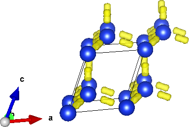
and open Si.xsf in VESTA to visualize the structure and electron density. (Adjust the boundary setting to 2 repetitions in each dimension to get the result shown above.) Note the tubes of electron density along nearest-neighbour Si atoms, forming a tetrahedral network (diamond lattice). Now set the boundary setting to 8 in each dimension to match the kpoint-folding. Intuitively, Brillouin zone sampling makes the wavefunctions periodic on this structure (with 512 unit cells and 1024 atoms), rather than on the much smaller unit cell with only 2 atoms.
Finally, let's examine how the total energy varies with Brillouin zone sampling. Edit the kpoint-folding line in Si.in to:
kpoint-folding ${nk} ${nk} ${nk}
so that we can script several calculations using variable substitution:
#!/bin/bash
for nk in 1 2 4 8 12 16; do
    export nk  #Export adds shell variable nk to the enviornment
               #Without it, nk will not be visible to jdftx below
    mpirun -n 4 jdftx -i Si.in | tee Si-$nk.out
done
listEnergy Si-?.out Si-??.out
Save the above to run.sh, execute "chmod +x run.sh", and then run using "./run.sh". At the end, it will list the energies for the different calculations:
-7.317807660097655 Si-1.out
-7.849193634824133 Si-2.out
-7.936090648821331 Si-4.out
-7.942846959204424 Si-8.out
-7.942984013789327 Si-12.out
-7.942989279183072 Si-16.out
Note that the energy converges rapidly after 8 kpoints per dimension, and the energy at 8 kpoints per dimension is only around 0.0001 Hartree away from that at 16 kpoints per dimension. The number of kpoints necessary for convergence varies from one system to another, and should be tested for each new material.
Above we worked with "kpoint 0 0 0 1." (issued automatically; last parameter is the weight), which on folding results in "Gamma-centered" kpoint meshes. Add the following line to Si.in:
kpoint 0.5 0.5 0.5 1.
which results in a mesh offset from the Gamma point, called the "Monkhost-Pack" mesh. Rerun the convergence test script to get the results:
-7.849461799239376 Si-1.out
-7.937020474685965 Si-2.out
-7.942892147278267 Si-4.out
-7.942989527101191 Si-8.out
-7.942989655201798 Si-12.out
-7.942989659123112 Si-16.out
which converges faster with number of kpoints per dimension. Notice however that each calculation had more symmetry-reduced kpoints now (grep nStates Si-?.out Si-??.out) compared to the Gamma-centered case, and hence ran slower.
Exercise: plot the energy convergence of both types of kpoint meshes together, as a function of nStates.