The previous tutorial showed one way of examining Kohn-Sham eigenvalues in a crystal, the electronic band structure, which plotted the eigenvalues along a path. This tutorial calculates the density of states in silicon, which is the probability distribution of eigenstates in energy (eigenvalue) space.

First, we calculate the total density of states using:

#Save to Si.in and run "mpirun -n 4 jdftx -i Si.in"
lattice face-centered Cubic 10.263
ion-species GBRV/$ID_pbe.uspp
elec-cutoff 20 100

ion Si 0.00 0.00 0.00  0
ion Si 0.25 0.25 0.25  0

kpoint-folding 12 12 12     #Use a Brillouin zone mesh
electronic-SCF              #Perform a Self-Consistent Field optimization
dump-name Si.$VAR
dump End None

elec-n-bands 10             #Si has 4 occupied bands; asking for 6 unoccupied bands
converge-empty-states yes   #Make sure that empty state eigenvalues are reliable

density-of-states Total     #Output total density-of-states

Starting from the total energy calculations of the previous two tutorials, all we needed to do is add the command density-of-states. Additionally, in order to get a few unoccupied states, we ask for more bands using elec-n-bands and make sure the empty states are converged at the end of the calculation using converge-empty-states. (Note that empty or unoccupied states that don't affect the total energy need not converge at all in a minimize calculation, and may not converge fully in an SCF optimization.) We also cranked up the number of k-points to get smoother results.

Running the above calculation produces a plain text file "Si.dos", which we can straightforwardly plot in gnuplot using the commands (interactively in the gnuplot terminal):

plot "Si.dos" u 1:2 w l

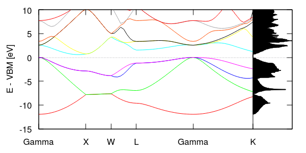
However, to make things a little more interesting (and show off some gnuplotting!), let's combine this with the band structure from the previous tutorial. Edit the last section of bandstruct.plot (including the edits from the previous tutorial) to be:

set xzeroaxis               #Add dotted line at zero energy
set ylabel "E - VBM [eV]"   #Add y-axis label
set yrange [*:10]           #Truncate bands very far from VBM
eV = 1/27.2114              #Value of eV in Hartrees
VBM = 0.227557              #VBM value (HOMO from totalE.eigStats)
xEnd = 68                   #Last x-tic value on k-path
set arrow \
  from first xEnd, graph 0 \
    to first xEnd, graph 1  #Draw separator

plot \
  for [i=1:nCols] "bandstruct.eigenvals" binary format=formatString u 0:((column(i)-VBM)/eV) w l, \
  "Si.dos" u (xEnd+0.2*$2):(($1-VBM)/eV) with filledcurves y1=xEnd linecolor rgb "black"

This rotates the density-of-states and aligns its energy with the y-axis of the band structure, producing the plot shown above. Note the correlations between features in the band structure and the density of states. The highest density occurs where there are bands with low curvature, such as the flat section of the lowest bands in the XW segment and the low curvature for the lowest unoccupied bands near Gamma. Can you identify the band gap in the density of states? Correlating it with the band structure, is it a direct or indirect band gap? (That is are the highest occupied and lowest unoccupied states at the same k-point, or different ones?)

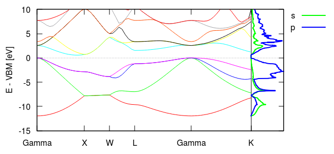
Next, let us examine contributions from various orbitals to the density of states. Modify the density-of-states commands in Si.in to:

density-of-states \
    OrthoOrbital Si 1 s \
    OrthoOrbital Si 1 p

and rerun jdftx on that input file. Here we requested s and p orbital-projected contributions, which will both be saved to columns in the same file Si.dos. Update the final section of the latest version of bandstruct.plot to:

set key top right outside
plot \
   for [i=1:nCols] "bandstruct.eigenvals" binary format=formatString u 0:((column(i)-VBM)/eV) w l title "", \
   "Si.dos" u (xEnd+0.5*$2):(($1-VBM)/eV) w l lw 2 title "s", \
   "Si.dos" u (xEnd+0.5*$3):(($1-VBM)/eV) w l lw 2 title "p"

and rerun "gnuplot --persist bandstruct.plot" to get the plot shown below. This time, instead of plotting a single total density of states, we plotted the contributions due to the s and p orbitals on the first Si atom. Note that the lower occupied bands exhibit s and p character, while the higher occupied bands have predominantly p character. The unoccupied bands have mixed character, but with a higher p fraction.