The solids discussed so far are bound together by strong bonds: covalent bonds in silicon, metallic bonds in platinum and iron, and covalent/ionic bonds in iron oxide. Density-functional theory is reasonably accurate for predicting the lattice and ionic geometries of such materials, but misses the weaker van der Waals (vdW) or dispersion interactions caused by long-range correlations of electron fluctuations. This tutorial illustrates this issue in graphite, and shows how to mitigate it using the DFT+D2 vdW correction.

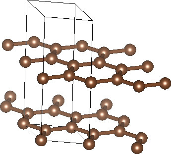
Graphite consists of layers of hexagonal carbon networks (graphene) with weak interlayer binding from van der Waals interactions. The two-dimensional unit cell for one hexagonal layer contains two carbon atoms. The layers alternate with one atom in line with those of neighbouring layers, and the other over the hexagonal voids of neighbouring layers. Vertically, a unit cell therefore includes two layers, with a total of four carbon atoms. Experimentally, the hexagonal lattice constants are a = 2.461 Angstroms (4.651 bohrs) and c = 6.708 Angstroms (12.676 bohrs), which correspond to in-plane carbon-carbon bond lengths of a/sqrt(3) = 1.42 Angstroms and interlayer spacing of c/2 = 3.35 Angstroms. We can setup a unit cell with the experimental geometry as:

#Save the following to graphite.lattice:
lattice Hexagonal 4.651 12.676


#Save the following to graphite.in:
include graphite.lattice
ion C  0.000000  0.000000  0.0   0
ion C  0.333333 -0.333333  0.0   0
ion C  0.000000  0.000000  0.5   0
ion C -0.333333  0.333333  0.5   0

ion-species GBRV/$ID_pbe.uspp
elec-cutoff 20 100
kpoint-folding 12 12 4

elec-smearing Fermi 0.01
electronic-SCF
lattice-minimize nIterations 10
dump End Lattice
dump-name graphite.$VAR

and optimize the lattice geometry using:

mpirun -n 4 jdftx -i graphite.in | tee graphite.out
mpirun -n 4 jdftx -i graphite.in | tee -a graphite.out

(continuing the calculation at least once to minimize basis-set errors as discussed in the Lattice optimization tutorial).

Check the final converged lattice constants: the in-plane directions expand by about 0.2% indicating that DFT is quite accurate for the strong covalent C-C bond lengths. However, the vertical direction expands by over 20% indicating that DFT severely underestimates the interlayer vdW interactions.

We can compensate for the missing vdW interactions using Grimme's DFT+D2 method which adds a pair-potential term using atomic polarizabilities with an empirical scale factor fit to the geometries of several vdW complexes. To use this in the code, add the command

van-der-waals

to the input file and rerun JDFTx a couple of times. Note that you start out at the previously-converged expanded unit cell (unless you reset grahite.lattice manually). After converging with these vdW corrections, the in-plane lattice constant is within 0.1% of the experimental value and the vertical lattice constant is approximately 5% smaller than experiment. Therefore, with the corrections, this DFT+D2 approach slightly overestimates the strength of the interlayer vdW interactions in graphene, but overall performs much better in absolute error than with no correction.

If highly accurate geometries are desired for a particular class of vdW-bound materials, it is possible to adjust either the overall scale factor using the van-der-waals command, or using the individual atom polarizabilities using the setVDW command. See the "Initializing van der Waals corrections" section of the output file to find the default values of C6 coefficients used for the atoms.

Exercises: find the optimum vdW scale factor for graphite using the default C6, and similarly find the optimum C6 using the default scale factor.