The previous tutorial introduced a basic calculation of a water molecule, and visualized one possible output: the electron density. This tutorial explores other possible outputs from the same calculation. It also discusses how to access the binary output files from Octave/MATLAB or Python/NumPy, which you can skip till later if/when you need to do custom postprocessing on JDFTx outputs.

Here's the same input file water.in as before, with the introductory comments removed, and with more output options requested:

lattice Cubic 10  #Alternate to explicitly specifying lattice vectors
elec-cutoff 20 100
ion-species GBRV/h_pbe.uspp
ion-species GBRV/o_pbe.uspp
coords-type cartesian     
ion O   0.00 0.00  0.00  0
ion H   0.00 1.13 +1.45  1
ion H   0.00 1.13 -1.45  1

dump-name water.$VAR              #Filename pattern for outputs

#Outputs every few electronic steps:
dump Electronic State        #The first parameter is when to dump, the remaining are what
dump-interval Electronic 5   #How often to dump; this requests every 5 electronic steps

#Output at the end:
dump End Ecomponents ElecDensity EigStats Vscloc Dtot RealSpaceWfns

Here we invoke the dump command multiple times to request different quantities to be output at various stages of the calculation. The dump-interval controls the interval at each type of calculation stage where output can be retrieved.

Now run

jdftx -i water.in | tee water.out

and examine water.out. Every 5 electronic steps, the calculation outputs State, which is the collection of all variables necessary to continue the calculation. In this case, that consists of wfns, the electronic wavefunctions (more precisely, Kohn-Sham orbitals) as can be seen in the repeated lines 'Dumping water.wfns ... done.'

After completing electronic minimization, the calculation dumps

Filename	Description
water.Ecomponents	Ecomponents (energy components)
water.eigStats	EigStats (eigenvalue statistics)
water.n	ElecDensity (electron density)
water.d_tot	Dtot (which is the net electrostatic potential)
water.Vscloc	Vscloc (which is the self-consistent Kohn-Sham potential)
water.wfns_0_x.rs	with x=0,1,2,3 for RealSpaceWfns (real-space wave functions)

Examine water.Ecomponents. It contains the energy components printed in exactly the same format as the output file. The energy components reported in this case are

Component	Description
Eewald	Ewald: nuclear-nuclear Coulomb energy
EH	Hartree: electron-electron mean-field Coulomb energy
Eloc	Electron-nuclear interaction (local part of pseudopotential)
Enl	Electron-nuclear interaction (nonlocal part of pseudopotential)
Exc	Exchange-Correlation energy
Exc_core	Exchange-Correlation energy subtraction for core electrons
KE	Kinetic energy of electrons
Etot	Total energy

Next look at water.eigStats (same content also reproduced in output file). It contains statistics of the Kohn-Sham eigenvalues such as the minimum and maximum, and the highest-occupied orbital (HOMO) energies. Some of the energies, such as the lowest-unoccupied orbital (LUMO) energy and electron chemical potential (mu) are reported as unavailable since the present calculation did not include any unoccupied states.

The remaining outputs are binary files containing the values of the corresponding quantities on a uniform grid, in this case on a 40 x 40 x 40 grid for the wavefunctions and a 48 x 48 x 48 grid for the remainder (see the lines starting with 'Chosen fftbox' in the initialization section of the output file).

Within the Octave or MATLAB commandline, we can examine the binary electron density file which contains the electron density n(r) at each grid point (in electrons/bohr³ units) using:

 fp = fopen('water.n', 'rb');  %# read as a binary file
 n = fread(fp, 'double');      %# stored as double-precision floating point numbers
 %# n = swapbytes(n);          %# uncomment on big-endian machines; data is always stored litte-endian
 fclose(fp);

 S = [ 48 48 48 ];             %# grid dimensions (see output file)
 V = 1000;                     %# unit cell volume (see output file)
 dV = V / prod(S);
 Nelectrons = dV * sum(n)

 n = reshape(n,S)(:,:,1);      %# convert to 3D and extract yz slice
 n = circshift(n, S(1:2)/2);   %# shift molecule from origin to box center
 contour(n)

This should print Nelectrons = 8, the number of valence electrons in the calculation and then present a contour plot of the yz slice of the electron density. Note that Octave/MATLAB differ from C++ in the array ordering convention, so the first array dimension is z, the second is y and the final one is x. The circshift prevents the tearing of the molecule across the boundaries. (The big-endian fix only applies if you are working on a PowerPC architecture, such as the Bluegene supercomputer and very old Macs; this is very unlikely.)

Alternately, if you prefer Python/NumPy, you can achieve exactly the same result with:

 import numpy as np
 import matplotlib.pyplot as plt

 n = np.fromfile('water.n',   # read from binary file
           dtype=np.float64)  # as 64-bit (double-precision) floats
 #n = swapbytes(n)            # uncomment on big-endian machines; data is always stored litte-endian

 S = [48,48,48]               # grid dimensions (see output file)
 V = 1000.0                   # unit cell volume (see output file)
 dV = V / np.prod(S)
 print "Nelectrons = ", dV * np.sum(n)

 n = n.reshape(S)[0,:,:]        # convert to 3D and extract yz slice
 n = np.roll(n, S[1]/2, axis=0) # shift molecule from origin to box center (along y)
 n = np.roll(n, S[2]/2, axis=1) # shift molecule from origin to box center (along z)
 plt.contour(n)
 plt.show()

The only difference here is that the default data order in NumPy is the same as C++.

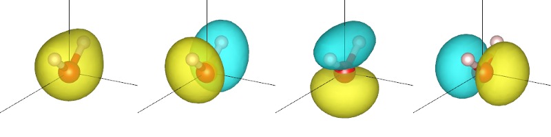
The above scripts show you how you can directly access the binary output data for custom post-processing and plotting. However, for simple visualization tasks, the createXSF script should suffice, as we demonstrated with the electron density at the end of the previous tutorial. Now visualize the Kohn-Sham orbitals using:

createXSF water.out water-x.xsf water.wfns_0_x.rs

for each x in 0,1,2,3, and view each of the generated XSF files using VESTA to get the plots shown below and at the start of this tutorial. (You will need to change the boundary setting as in the previous tutorial.)

The orbitals are sorted by their corresponding energy eigenvalue. In VESTA, the yellow and cyan correspond to different signs of the plotted quantity. Note that the lowest orbital has the same sign thoughout, whereas the remaining three have symmetric positive and negative regions separated by a nodal plane (where the orbital is zero). Two of the three nodal planes are exact planes constrained by reflection symmetry of the molecule, while the third is only approximately a plane. (Which one is that?)