 |
JDFTx
1.7.0
|


|
|
JDFTx
1.7.0
|
|
| 
|
This tutorial introduces the setup of more complex surfaces, and demonstrates bound charge and electrostatic potential visualization, using the example of Rutile TiO2(110) in vacuum and solution.
Let's start with a calculation of the bulk titanium dixoide, which has a Rutile crystal structure consisting of a tetragonal unit cell with parameters a = 4.59 Angstroms (8.67 bohrs) and c = 2.96 Angstroms (5.59 bohrs). Each unit cell contains two TiO2 units, with one Ti at a vertex and the other at the body center. To speed up the calculations, we skip geometry optimization in this tutorial, and I directly list the optimized ionic positions below.
#Save the following to bulk.in:
ion-species GBRV/$ID_pbe.uspp
elec-cutoff 20 100

lattice Tetragonal 8.67 5.59
ion Ti   0.5000 0.5000 0.5   1
ion Ti   0.0000 0.0000 0.0   1
ion  O   0.6958 0.6958 0.0   1
ion  O   0.8042 0.1958 0.5   1
ion  O   0.3042 0.3042 0.0   1
ion  O   0.1958 0.8042 0.5   1

kpoint-folding 4 4 6   #Less kpoints along longer lattice vectors
electronic-SCF
dump End None
Run jdftx on bulk.in, use createXSF to generate bulk.xsf and visualize it using VESTA, as usual.
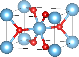
Note that each Ti atom is surrounded by six O atoms in a (distorted) octahedron, and that each O atom connects to three Ti atoms in a plane. Record the total energy of the bulk unit cell, as we will need it later for calculating surface energies.
We will follow the procedure introduced in the Pt(100) setup page to setup the surface geometry, with a few additions to account for the differences. This time, we will make a slab with three layers (to keep the calculations quicker) and include a vacuum spacing of approximately 15 bohrs as before. For production calculations, converge the results with number of layers.
The original tetragonal lattice vectors (in columns) are:
    / a 0 0 \
R = | 0 a 0 |
    \ 0 0 c /
The 110 surface normal must combine the first two lattice vectors (this time the third axis is different from the first two) with equal coefficients, leading to the obvious choice [ 1 1 0 ]. We now need two perpendicular directions for the in-plane superlattice vectors. Note that [ -1 1 0 ] is a combination of the first two lattice vectors which is perpendicular to the chosen surface normal. The third lattice vector is already normal to both of these, so can become a superlattice vector unmodified (combination [ 0 0 1 ]). Therefore, we arrive at the transformation matrix (above combinations in columns):
    / -1  0  1 \
M = |  1  0  1 |
    \  0  1  0 /
and the resulting superlattice vectors:
                / -a  0  a \
Rsup = R . M =  |  a  0  a |
                \  0  c  0 /
The supercell has twice the volume of the unit cell since det(M) = 2, and therefore we need two copies of the atoms. We can take the original atom coordinates and transform them to supercell fractional coordinates by multiplying by inv(M):
ion Ti   0.0000  0.5  0.5000  1
ion Ti   0.0000  0.0  0.0000  1
ion  O   0.0000  0.0  0.6958  1
ion  O  -0.3042  0.5  0.5000  1
ion  O   0.0000  0.0  0.3042  1
ion  O   0.3042  0.5  0.5000  1
For the second set of atoms, we add an offset of [ 1 0 0 ] in the original lattice coordinates (any original lattice vector that has a component along the surface normal will work), which upon multiplying by inv(M), becomes an offset of [ -1/2 0 1/2 ] in the superlattice coordinates. Putting together the second set of atoms with this offset, wrapping all coordinates into the range [0,1) using periodicity, and sorting atoms by the third coordinate, we get:
ion Ti   0.0000  0.0  0.0000  1
ion Ti   0.5000  0.5  0.0000  1
ion  O   0.1958  0.5  0.0000  1
ion  O   0.8042  0.5  0.0000  1
ion  O   0.5000  0.0  0.1958  1
ion  O   0.0000  0.0  0.3042  1

ion Ti   0.0000  0.5  0.5000  1
ion Ti   0.5000  0.0  0.5000  1
ion  O   0.6958  0.5  0.5000  1
ion  O   0.3042  0.5  0.5000  1
ion  O   0.0000  0.0  0.6958  1
ion  O   0.5000  0.0  0.8042  1
Note that this looks like two layers consisting of two TiO2 units each, which is what we need in order to cleave and get a surface. However note that each layer is lopsided: it consists of two Ti and two O atoms all with the same third coordinate (0.0 or 0.5 depending on the layer), and the remaining two O atoms to the same side of this sheet, one closer and the other further away. By wrapping the third coordinate of the last O atom using periodicity, we can make both layers symmetric with one O atom above and below each Ti2O2 sheet:
ion  O   0.5000  0.0 -0.1958  1
ion Ti   0.0000  0.0  0.0000  1
ion Ti   0.5000  0.5  0.0000  1
ion  O   0.1958  0.5  0.0000  1
ion  O   0.8042  0.5  0.0000  1
ion  O   0.5000  0.0  0.1958  1

ion  O   0.0000  0.0  0.3042  1
ion Ti   0.0000  0.5  0.5000  1
ion Ti   0.5000  0.0  0.5000  1
ion  O   0.6958  0.5  0.5000  1
ion  O   0.3042  0.5  0.5000  1
ion  O   0.0000  0.0  0.6958  1
Two layers have thickness sqrt(2)a (the third superlattice vector length) = 12.26123 bohrs, so three layers occupy approximately 18.4 bohrs. We will make the net unit cell height 33 bohrs to include 15 bohrs vacuum spacing, which requires scaling the third atom fractional coordinates by 12.26123/33 = 0.37155, and offsetting layers by the same amount. By selecting three layers symmetrically about zero, we arrive at the geometry:
#Save the following to Rutile110.ionpos:
ion  O   0.0000  0.0 -0.25852  1
ion Ti   0.0000  0.5 -0.18578  1
ion Ti   0.5000  0.0 -0.18578  1
ion  O   0.6958  0.5 -0.18578  1
ion  O   0.3042  0.5 -0.18578  1
ion  O   0.0000  0.0 -0.11303  1

ion  O   0.5000  0.0 -0.07275  1
ion Ti   0.0000  0.0  0.00000  1
ion Ti   0.5000  0.5  0.00000  1
ion  O   0.1958  0.5  0.00000  1
ion  O   0.8042  0.5  0.00000  1
ion  O   0.5000  0.0  0.07275  1

ion  O   0.0000  0.0  0.11303  1
ion Ti   0.0000  0.5  0.18578  1
ion Ti   0.5000  0.0  0.18578  1
ion  O   0.6958  0.5  0.18578  1
ion  O   0.3042  0.5  0.18578  1
ion  O   0.0000  0.0  0.25852  1
with the lattice vectors:
#Save the following to Rutile110.lattice:
lattice Orthorhombic 12.26123 5.59 33   #Respectively sqrt(2)a, c and chosen height with spacing
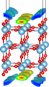
Use testGeometry.in from the Pt(100) setup page to visualize the geometry via a JDFTx dry run. You should see a structure as shown at the top of the page (except without the bound charge distributions, which we will calculate below).
Now we can create input files for vacuum and solvated surface calculations, exactly as in the Metal surfaces tutorial, with a few minor tweaks: we can use fewer k-points and don't need Fermi fillings since this is an insulator, and we will output electrostatic potentials and bound charge for visualization.
#Save the following to common.in:
include Rutile110.lattice
include Rutile110.ionpos
ion-species GBRV/$ID_pbe.uspp
elec-cutoff 20 100
coulomb-interaction Slab 001
coulomb-truncation-embed 0 0 0
kpoint-folding 3 6 1       #Chosen in inverse proportion to lattice vector length
lcao-params 30             #More initialization steps for a better starting point
electronic-SCF


#Save the following to Vacuum.in:
include common.in
dump-name Vacuum.$VAR
dump End State Dtot


#Save the following to Solvated.in:
include common.in
initial-state Vacuum.$VAR
dump-name Solvated.$VAR
dump End Dtot BoundCharge
fluid LinearPCM
pcm-variant CANDLE
fluid-solvent H2O
fluid-cation Na+ 1.
fluid-anion F- 1.
Then run both the vacuum and solvated calculations (these will take a while):
jdftx -i Vacuum.in | tee Vacuum.out
jdftx -i Solvated.in | tee Solvated.out
createXSF Solvated.out Solvated.xsf nbound
and visualize the resulting XSF file with VESTA to see the structure with the bound charge distribution in the solvent (as shown at the top of this page, after adjusting the boundary setting in VESTA as described previously). Notice the positive bound charge near the oxygen bridges at the surface and the negative bound charge in the solvent near the exposed Ti atoms at the surface.
Adapt collectResults.sh from the Metal surfaces tutorial to extract and report the surface energies in vacuum and solution. In this case, we do not have electron chemical potential (mu) output to track because we disabled Fermi fillings. To understand the effect of band positions, we could instead use the EigStats output and compare the VBM (HOMO) energies. For demonstration purposes, however, we will extract the solvation shift from the total electrostatic potential (Dtot) output instead, as described in the next section.
| Model | Esurf [eV/nm2] | VBM shift [eV] | ||
|---|---|---|---|---|
| Vacuum | Solvated | Shift | ||
| CANDLE | 8.58 | 6.78 | -1.80 | 1.04 |
| GLSSA13 | 2.50 | -6.08 | 3.15 | |
Note that the surface energy reduction due to solvent stabilization is much larger compared to the metal surface case because of the positive (Ti) and negative (O) charge regions on the surface. The VBM shift predicted by CANDLE (extracted using the scripts below) is in good agreement with experimental estimates (0.9-1.1 eV). But this agreement is somewhat fortuitous: converging the result with number of layers and geometry opimization lowers the predicted shift to 0.6 eV and worsens agreement somewhat. See Refs. [33] and [3] for further discussion of energy level alignment in oxide-water interfaces.
For comparison, I also show results for the GLSSA13 LinearPCM (same as VASPsol, similar to SCCS). Note that those solvation models have two fundamental difficulties with oxide surfaces resulting in poor convergence and unphysical results:
By starting from the non-empirical and nonlocally-determined SaLSA cavity, CANDLE and SaLSA address both these issues. The non-locality ensures that an entire water molecule must fit in the voids, significantly minimizing the probability of unphysical leakage. Additionally, the density-product cavity determination is calibrated to work on all atoms in the periodic table, and not just organic solutes.
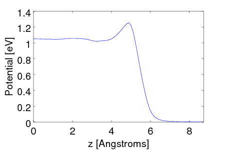
We will now extract the electrostatic potential output from both the vacuum and solvated calculations (Vacuum.d_tot and Solvated.d_tot). The difference between these electrostatic potentials goes to zero far away from the slab, and approaches a constant value towards the center of the slab. This potential shift in the center fo the slab corresponds to the shift in the bulk energy levels of the solid due to the interfacial potential at the solid-liquid interface, which is the solvation VBM shift we seek.
The following python script extracts the potentials, planarly averages them perpendicular to the slab normal (z) direction, plots the difference and reports the VBM shift.
import numpy as np
import matplotlib.pyplot as plt

S = [ 56, 28, 160 ]            #Sample count (fftbox from log file)
L = [ 12.26123, 5.59, 33. ]    #Lattice vector lengths (bohrs)
z = np.arange(S[2])*L[2]/S[2]  #z-coordinates of grid points

def readPlanarlyAveraged(fileName, S):
    out = np.fromfile(fileName, dtype=np.float64)
    out = np.reshape(out, S)   #Reshape data
    out = np.mean(out, axis=1) #y average
    out = np.mean(out, axis=0) #x average
    return out

dVacuum = readPlanarlyAveraged('Vacuum.d_tot',S)
dSolvated = readPlanarlyAveraged('Solvated.d_tot',S)
dShift = dSolvated - dVacuum

print "VBMshift =", dShift[0]*27.2114  #Report VBM shift in eV
plt.plot(z*0.529, dShift*27.2114);     #Plot with unit conversions
plt.xlabel('z [Angstroms]')
plt.ylabel('Potential [eV]')
plt.xlim([0, L[2]/2*0.529])            #Select first half (top surface only)
plt.show()
This Octave/MATLAB script achieves the same result, with some minor differences due to data ordering:
S = [ 56 28 160 ];          %Sample count
L = [ 12.26123 5.59 33 ];   %Lattice vector lengths (bohrs)
z = [0:S(3)-1]*L(3)/S(3);   %z-coordinates of grid points

function out = readPlanarlyAveraged(fileName, S)
    %Read data:
    fp = fopen(fileName, 'r');
    out = fread(fp, 'double');
    fclose(fp);
    out = reshape(out, fliplr(S)); %Reshape data (flipped order)
    out = mean(mean(out,2),3);     %xy average (flipped order)
end

dVacuum = readPlanarlyAveraged('Vacuum.d_tot',S);
dSolvated = readPlanarlyAveraged('Solvated.d_tot',S);
dShift = dSolvated - dVacuum;

VBMshift = dShift(1)*27.2114   %Report VBM shift in eV
plot(z*0.529, dShift*27.2114); %Plot with unit conversions
xlabel('z [Angstroms]');
ylabel('Potential [eV]');
xlim([0 L(3)/2]*0.529);        %Select first half (top surface only)
pause
The resulting potential plot is shown at the top of the page. Note the oscillating response in the outer layers of the slab which decays towards the constant value in the center.