All the calculations so far have been of isolated molecules in vacuum, which is a good description for dilute gases. However, chemical reactions often occur in a solution, and predicting reaction mechanisms using DFT requires calculating structures and free energies of molecules in solution. Directly describing the solvent using its constituent molecules requires several thousands of DFT calculations to sample all configurations of solvent molecules, and is extremely computationally intensive. A practical alternative is to use a continuum solvation model which directly approximates the equilibrium effect of the solvent on a solute, without treating individual solvent configurations.

A major focus in the development of JDFTx has been the development of a heirarchy of solvation models from continuum to a detailed classical DFT approach, within the framework of Joint Density Functional Theory. (That's where JDFTx gets its J!) This tutorial shows how to put molecules in solution and introduces some of the commands that control solvation and fluid properties.

Let's put a water molecule in liquid water. The free energy of this process is related to the vapor pressure of liquid water and can be calculated from experimental measurements as -0.0101 Hartrees (= -6.33 kcal/mol). First, we perform the calculation in vacuum using the input files

#Save to common.in
lattice Cubic 15
coulomb-interaction Isolated
coulomb-truncation-embed 0 0 0
ion-species GBRV/$ID_pbe.uspp
elec-cutoff 20 100
coords-type cartesian

containing the shared commands as before, and

#Save to Vacuum.in and run as jdftx -i Vacuum.in | tee Vacuum.out:
include common.in
ion O   0.00 0.00  0.00  0
ion H   0.00 1.13 +1.45  1
ion H   0.00 1.13 -1.45  1
ionic-minimize nIterations 10
dump-name Vacuum.$VAR
dump End State

Upon completion, this calculation will output the optimized geometry and wavefunctions of a water molecule in vacuum. Next, we run a solvated calculation starting from this state:

#Save to LinearPCM.in and run as jdftx -i LinearPCM.in | tee LinearPCM.out:
include common.in
include Vacuum.ionpos
initial-state Vacuum.$VAR
ionic-minimize nIterations 10
dump-name LinearPCM.$VAR
dump End State BoundCharge

fluid LinearPCM     #Simple continuum fluid with linear response
pcm-variant GLSSA13 #default, if not specified
fluid-solvent H2O   #Solvent is water

This runs a solvated calculation with the simplest GLSSA13 LinearPCM model (this is exactly the same model which was later implemented in VASP as VASPsol) and outputs the bound charge density induced in the solvent by electrostatic interactions with the solute. Examine the output file: now there are lines starting with 'Linear fluid' between electronic steps. These correspond to optimization of the fluid degrees of freedom (in this simple case, by solving a linearized Poisson-Boltzmann equation) in response to the solute's charge density. The energy components now include an additional piece Adiel, which is the total contribution due to the solvent.

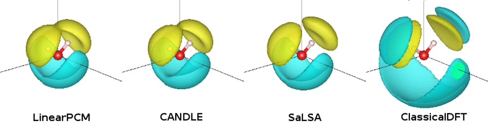
The solvation free energy is the difference between the final energies in Vacuum.out and LinearPCM.out, which turns out to be (-17.2682) - (-17.2795) = -0.0113 Hartrees in good agreement with the experimental estimate of -0.0101 Hartrees. Visualizing the bound charge density (nbound) using

createXSF LinearPCM.out LinearPCM.xsf nbound

results in the first panel of the figure above.

The command fluid selects the broad class of solvation model, some of which support many variants selected by command pcm-variant. Some of the common / recommended models are:

LinearPCM (GLSSA13): This default LinearPCM is currently the most popular solvation model in solid-state calculations, especially in the form of the VASPsol solvation module in the proprietary DFT software VASP. In this simple solvation model, the liquid responds with induced charge densities at the surface of a dielectric cavity surrounding the solute molecule, and this cavity in turn is determined as a function of the solute electron density. This solvation model is selected by the following commands, as described above:
```
fluid LinearPCM
pcm-variant GLSSA13
```
SCCS: The self-consistent continuum solvation (SCCS) method is closely related to the default LinearPCM and primarily differs in the details of the function that determines the cavity from the electron density. This is the solvation model available in the Quantum Espresso DFT software. There are several parametrizations of this model, all with names starting with SCCS (see command pcm-variant):
```
fluid LinearPCM
pcm-variant SCCS_*
```
CANDLE This is the latest solvation model and recommended for most applications. It has the computational expense of the simpler LinearPCM's above but incorporates the accuracy and robustness of the more expensive models discussed next. In summary it uses SaLSA's nonlocal electron-density overlap method to determine the cavity, but then uses a local dielectric response like other LinearPCM's. It additionally corrects for the asymmetry in the response of the liquid to positively and negatively charged solutes.
```
fluid LinearPCM
pcm-variant CANDLE
```
NonlinearPCM: This class of solvation models captures the nonlinearity in the dielectric and ionic response of the solvent. This is necessary if you need to capture details in the capacitance of electrochemical systems, for example.
```
fluid NonlinearPCM
pcm-variant GLSSA13
```
SaLSA: This solvation model directly captures the nonlocal response of the liquid using an angular mometum expansion (not continuum like the rest), and determines the cavity from an overlap of solute and solvent electron densities. This model is typically a factor of 10 more expensive than the continuum solvation models. Usually CANDLE, which empirically mimics the SaLSA response, should suffice, but SaLSA is a parameter-free physically-motivated model that is a useful benchmark for the more empirical methods like CANDLE in new / untested classes of solutes.
```
fluid SaLSA
```
ClassicalDFT: A full classical DFT description of the fluid is used to fully capture the microscopic structuring of the liquid at the atomic scale. This method is typically a factor of 100 more expensive than the continuum methods, but is the only method that provides access to liquid structure in the solvent in addition to the electronic structure of the solute. This is particularly useful for analyzing in-situ structure measurements (eg. X-ray) of electrochemical interfaces. See commands fluid-solvent for controlling details of the solvent ClassicalDFT such as orinetation sampling and fluid-gummel-loop to control the self-consistency algorithm that optimizes the liquid and electronic states. With default options, all it takes to use it is the command:
```
 fluid ClassicalDFT
```
Also see the various commands listed under fluid in the Input file documentation page for controlling numerous details of the fluid calculation.

Now, as an exercise run the water calculation with each class of solvation model, compare the solvation energies and visualize the bound charge in the liquid using createXSF and VESTA, as shown below and at the start of this tutorial. (SaLSA and ClassicalDFT will take a while!) Note how LinearPCM, the nonlocally-inspired variant CANDLE, as well as the non-local model SaLSA have the bound charge mostly restricted to a surface surrounding the solute, whereas ClassicalDFT, exhibits a shell structure with several layers surrounding the solute. Additionally, in this simple case of a neutral solute, all the solvation models are comparably accurate.