This tutorial introduces the framework for computing the CD of a crystalline system. Previous theoretical methods employ a sum-over-states identity with momentum eigenvalues to calculate the CD. Our novel approach directly computes the orbital angular momentum (L) and electric quadripole (Q) matrix elements, which are then used in a post-processing script to find the CD signal (see [https://doi.org/10.48550/arXiv.2303.02764] for theoretical background).

For our system, we choose chiral metal CoSi due to the simplicity of its unit cell, though the computational framework can be generalized to any crystalline system of arbitrary unit cell complexity. This can also be applied to molecules, given they are placed in a box of sufficient size.

Beginning from a self-consistent energy density calculation, we use Monte-Carlo sampling to ensure an even sampling of the Brillouin Zone. To do so, we create 10 directories, each corresponding to a block of k-points, labeled "block_1", etc. Each block contains a "sampling.kpoints.in" file which contains a unique set of 250 randomly-generated k-points. We use a total of 2,500 k-points for sampling this system, though each system should be tested for convergence with respect to sampled k-points.

Each block also contains the input file, sampling.in:

include ../totalE.lattice
include ../totalE.ionpos
include sampling.kpoints.in

ion-species GBRV/$ID_pbe.uspp
elec-cutoff 50
elec-ex-corr gga-PBE

#Computing enough DFT bands to cover a desired energy range
elec-n-bands 100

#Fix the electron density (not self-consistent)
fix-electron-density ../totalE.$VAR

#Parameters specific to calculating finite difference derivative. Should be checked for each system
Cprime-params 7E-4
electronic-minimize energyDiffThreshold 5e-9
     
dump End BandEigs Momenta L Q BandProjections
dump-name bandstruct.$VAR

which can be run using:

mpirun -n 4 jdftx -i sampling.in | tee sampling.out

Once done, each block should now contain the necessary components for calculating CD: the energies (bandstruct.eigenvals), momentum (bandstruct.momenta), orbital angular momentum (bandstruct.L), and quadrupole (bandstruct.Q) matrix elements. The bandstruct.BandProjections file can be dumped optionally if one wants to decompose the CD signal into individual orbital contributions.

After the sampling job has been completed for each block of k-points, the internal CD script included in JDFTx can be used to compile the data and compute the CD.

This script contains the following input flags:

--dmu, the change in mu relative to mu (if available), or VBM of DFT calculation [eV] (required)
--n_blocks, the number of blocks of k-points (required)
--n_bands, the number of computed DFT bands (required)
--domega, the bin size for histogramming [eV] (optional)
--omegaMax, the frequency cutoff of CD signal [eV] (optional)
--T, the temperature at which to compute CD [K] (optional)
--omegaAnalysis, the frequencies at which to decompose the CD signal into organic/inorganic/mixed contributions [eV] (optional)

To compute CD using default settings of domega=0.1eV, omegaMax=10eV, T=298K, and no frequencies for analysis, we can run:

CD --dmu 0 --n_blocks 10 --n_bands 100

which will output the computed CD in CDpy_10_100.dat (or, generally, CDpy_{n_blocks}_{n_bands}.dat). Note that this data file contains the CD tensor at each energy value from 0 to omegaMax, with spacing of domega. The header of the data file shows the order of the listed values for each row, with the first being the energy value and the following six being the six directional components of the tensor. Note that the output CD signal is in units of inverse Naperian length. See [https://doi.org/10.48550/arXiv.2303.02764] for unit conversion to standard molar circular dichroism.

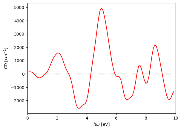
We can plot the CD signal using a simple python script:

#!/usr/bin/env python
import numpy as np
import matplotlib.pyplot as plt
from scipy.ndimage import gaussian_filter1d

CD = np.loadtxt('CDpy_10_100.dat')
omega = CD[:,0]

plt.plot(omega, gaussian_filter1d(CD[:,1],2), color='r')
plt.axhline(0., color='k', ls='dotted', lw=1)
plt.xlim(0., 10.)
plt.xlabel(r'$\hbar\omega$ [eV]')
plt.ylabel(r'CD [$cm^{-1}$]')
plt.legend(loc='upper left', bbox_to_anchor=(1,1))

plt.savefig('CD.png', bbox_inches='tight')
plt.show()