The previous tutorial showed a water molecule calculation in a cubic box of side 10 bohrs. JDFTx is a plane-wave DFT code, which means that it naturally incorporates periodic boundary conditions. However, for molecules we usually want to calculate the properties of one isolated molecule without incurring interactions between the molecule and its periodic images. JDFTx can eliminate image interactions in general geometries, for molecules, nanowires, slabs etc. using truncated Coulomb potentials. (See command coulomb-interaction.) This tutorial shows you the most convenient and efficient way to set up molecule calculations, starting from molecule geometries in the XYZ format, often used by the chemistry community.

Let's stick to water, but this time fetch the geometry from the NIST CCCBDB database. Picking one of the many calculated geometries of water from that database, we can create water.xyz containing:

3

O    0  0        0.127118
H    0  0.75799 -0.50847
H    0 -0.75799 -0.50847

The first line is the number of atoms, the second line is a comment line that is ignored, and the subsequent lines specify the atom type and cartesian coordinates in Angstroms.

Now, we can use the script xyzToIonposOpt from the JDFTx scripts directory to convert this to JDFTx input (see Getting started to add this directory to your run PATH, or specify full path to script below):

xyzToIonposOpt water.xyz 15

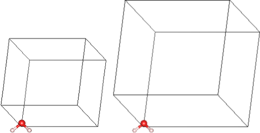
This script outputs ionic positions in water.ionpos and lattice vectors in water.lattice after centering the molecule at the origin and rotating it such that you can use the smallest box with a periodic image distance of 15 bohrs. Using these outputs, we can create the input file water.in:

include water.lattice
include water.ionpos
coords-type cartesian

ion-species GBRV/$ID_pbe.uspp        #Replace $ID by any atom symbol to find a pseudopotential
elec-cutoff 20 100                   #Recommended cutoffs for GBRV pseudopotentials
dump End None                        #Don't output anything for this example

which we can run as

jdftx -i water.in | tee water.out

In this input file, we specified the entire set of GBRV pseudopotentials using the wildcard syntax of command ion-species instead of selecting O and H pseudopotentials specifically. Therefore, we could replace water with another molecule containing other atom types with almost no change to the input file, making it extremely easy to set up similar calculations for a large number of molecules. Now, check the final energy of the water molecule (in Hartrees) using the script:

listEnergy water.out

Next, check how the energy changes upon increasing the box size. Replace 15 with 20, 25 and then 30 in xyzToIonposOpt above, and rerun jdftx and listEnergy for each. You could do this manually, but could easily script all these calculations in the bash shell and retrieve their energies using:

#!/bin/bash
for padding in 15 20 25 30; do
    xyzToIonposOpt water.xyz $padding
    jdftx -i water.in | tee water-$padding.out
done
listEnergy water-*.out

Note that you could directly type the above in the shell, or save them to a file, say run.sh, give execute permissions using chmod +x run.sh and then execute using ./run.sh

Finally, also add the coulomb trunaction commands to the above water.in:

coulomb-interaction Isolated         #Switch from periodic to isolated images mode
coulomb-truncation-embed 0 0 0       #Center of molecule; origin for breaking periodicity

and once again run the calculation for the four box sizes.

I get the following energies with and without Coulomb truncation for the different box sizes:

Padding	Without truncation	With truncation
15	-17.268078941702573	-17.267860822043808
20	-17.268005076655513	-17.267899023265009
25	-17.267959775753003	-17.267901318302076
30	-17.267937318025449	-17.267901948787543

Note that the energy converges much faster with box size after including truncation. In fact, with truncation, the energy converges exponentially with unit cell size, compared to an inverse-cubic convergence without truncation due to dipole-dipole interactions.

In this example, the energy with 15 bohr spacing with Coulomb truncation is within 5x10^-5 Hartrees of the value converged with box size, whereas a 30 bohr spacing is required to achieve that accuracy without truncation. Note that the calculation with the 30 bohr spacing is roughly 8 times slower than that with the 15 bohr spacing, so using optimized unit cells with truncated Coulomb interactions can substantially speed up your calculation.