 |
JDFTx
1.7.0
|


|
|
JDFTx
1.7.0
|
|
JDFTx is an electronic density-functional theory (DFT) software, which means that its primary functionality is to calculate the quantum-mechanical energy of electrons in an external potential, typically from nuclei (ions) in a molecule or solid. Specifically, the underlying theory is Kohn-Sham DFT which involves solving the single-particle Schrodinger equation in a self-consistent potential determined from the electron density. This tutorial demonstrates a DFT calculation of the energy and electron density of a water molecule.
A lot of effort in the research behind JDFTx has involved water: its dielectric response, equation of state, free energy functional etc. Therefore, a water molecule is a fitting first calculation. Save the following to water.in:
# The input file is a list of commands, one per line
# The commands may appear in any order; group them to your liking
# Everything on a line after a # is treated as a comment and ignored
# Whitespace separates words; extra whitespace is ignored
# --------------- Water molecule example ----------------

# Set up the unit cell - each column is a bravais lattice vector in bohrs
# Hence this is a cubic box of side 10 bohr (Note that \ continues lines)
lattice \
    10 0  0 \
    0  10 0 \
    0  0  10

elec-cutoff 20 100    #Plane-wave kinetic energy cutoff for wavefunctions and charge density in Hartrees

# Specify the pseudopotentials (this defines species O and H):
ion-species GBRV/h_pbe.uspp
ion-species GBRV/o_pbe.uspp

# Specify coordinate system and atom positions:
coords-type cartesian       #the other option is lattice (suitable for solids)
ion O   0.00 0.00  0.00  0  # The last 0 holds this atom fixed
ion H   0.00 1.13 +1.45  1  # while the 1 allows this one to move
ion H   0.00 1.13 -1.45  1  # during ionic minimization

dump-name water.$VAR              #Filename pattern for outputs
dump End Ecomponents ElecDensity  #Output energy components and electron density at the end
This input-file illustrates the bare minimum commands needed to set up a calculation. The lattice and ion commands set up the unit cell and geometry, and elec-cutoff controls the resolution of the plane-wave basis that is used to represent the wavefunctions and densities. See Input file documentation for a list of all available input file commands and their options.
In a plane-wave basis, bare nuclei are replaced by an effective potential due to the nucleus and core electrons, termed the pseudopotential, and only the remaining valence electrons are included explicitly in the DFT calculation. The ion-species commands select the GBRV pseudopotentials distributed with JDFTx. These are installed to the build directory, and JDFTx will automatically look for them there. If you use pseudopotentials not built into JDFTx, specify the absolute or relative paths instead. See the Pseudopotentials page for supported pseudopotential formats, other sets of pseudopotentials distributed with JDFTx, and a wildcard syntax for selecting an entire set of pseudopotentials (which we shall use henceforth).
Now, that basic input file can be run with
jdftx -i water.in -o water.out
That should complete in a few seconds and create files water.out, water.Ecomponents and water.n. Note that the default behavior of jdftx is to concatenate output files. If you wish to overwrite a previous water.out file, then add option -d to the command line.
Have a look at water.out. It lists the commands that were issued in the input file along with several more which have sensible defaults. For instance, the exchange functional defaults to GGA (elec-ex-corr gga-PBE). To use LDA instead, you would add command elec-ex-corr lda to the input file. Other commands do not have defaults, such as van-der-waals to include dispersion interactions which standard DFT functionals miss (discussed later in Dispersion (vdW) corrections tutorial); so don't forget to see Input file documentation for the full list of available commands.
The commands section is followed by initialization of the plane-wave grid, symmetries, pseudopotentials etc., and then the electronic minimization which logs the progress of the conjugate gradients minimizer (lines starting with ElecMinimize). The default is to minimize for 100 iterations or an energy difference between consecutive iterations of 10-8 Hartrees, whichever comes first. This example converges to that accuracy in around 15 iterations. Note that the ions have not been moved and the end of the output file lists the forces at the initial position.
Additional output files are written based on the options provided by the dump command. Here, we have requested a dump of energy components (in water.Ecomponents) and electron density (in water.n) at the end of the run, with filenames specified by dump-name.
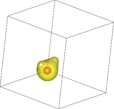
Finally, let's visualize the electron density output by this calculation. Use the createXSF script to create water.xsf containing the ionic geometry (extracted from water.out) and electron density (from water.n):
createXSF water.out water.xsf n
Note that the script recognizes dump-name, so n will be understood to be water.n, but you can also specify the file name directly. Now open the XSF file using the visualization program VESTA (or another program that supports XSF such as XCrysDen). You should initially see the water molecule torn between the corners of the box since it was centered at [0,0,0]. Change the visualization boundary settings from [0,1) to [-0.5,0.5) to see the (intact molecule) image at the top of the page!