All our caculations thus far have been for spin-neutral systems, with the exception of the hydrogen atom. This tutorial showcases spin-polarized calculations for crystalline solids using the archetypal example: metallic iron.

Iron has a body-centered cubic structure with a cubic lattice constant of 2.87 Angstroms (5.42 bohrs). Not surprisingly, we can set up an iron calculation using:

#Save the following to totalE.in:
lattice body-centered Cubic 5.42
ion-species GBRV/$ID_pbesol.uspp
elec-ex-corr gga-PBEsol
elec-cutoff 20 100
ion Fe  0 0 0  0
dump-name totalE.$VAR
dump End ElecDensity
density-of-states Total
kpoint-folding 12 12 12
elec-smearing Fermi 0.01
electronic-SCF

spintype z-spin                  #Allow up/dn spins (non-relativistic)
elec-initial-magnetization 3 no  #Initial guess, no = don't constrain

and run as usual using

mpirun -n 4 jdftx -i totalE.in | tee totalE.out

Note that the input file is very similar to platinum from the previous tutorial. Of course, we specified body-centered cubic instead of face-centered cubic, updated the lattice constant and the element name. We requested density-of-state and electron density output.

The key difference is the specification of spintype and elec-initial-magnetization, which we previously encountered in the Open-shell systems tutorial. This time, however, we specified no for the <constrain> parameter for the initial magnetization command, which allows it to be optimized when Fermi fillings are calculated. (Try it with yes and contrast the results!)

Examine the output file. During initialization, 48 symmetries are detected, which reduces the 12³ = 1728 input kpoints to 72 symmetry-reduced kpoints. However, nStates is now 2 x 72 = 144 due to the explicit treatment of spin.

The FillingsUpdate lines now additionally report magnetic moments of the system: Tot is the net magnetization of the unit cell, whereas Abs is the integral of the absolute value of the magentization density. For ferromagnetic iron, these two are similar, but in an antiferromagnet for example, Tot will be zero while Abs is finite. If both Tot and Abs turned out to be almost zero, it would have meant that the system prefers to be non-magnetic and that allowing for spin polarization (z-spin) should not be necessary. Also note that per atom magnetizations (and charges) are estimated in the Lowdin analysis (printed soon after each IonicMinimize line).

Finally, examine the output files dumped by the code at the end. For ElecDensity, it output n_up and n_dn instead of a single n. Similarly, the density of states for up and dn spins are split between two files totalE.dosUp and totalE.dosDn (instead of totalE.dos).

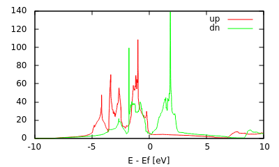
We can plot the density of states of the two spin channels together using the gnuplot script:

#!/usr/bin/gnuplot --persist
set xrange [-10:10]
set xlabel "E - Ef [eV]"
mu = 0.6377     #From the final FillingsUpdate line
eV = 1/27.2114
plot \
   "totalE.dosUp" u (($1-mu)/eV):2 w l title "up", \
   "totalE.dosDn" u (($1-mu)/eV):2 w l title "dn"

as shown at the top of the page.

Note that the up and down spins have very similar shapes in their density of states, but they are offset relative to each other. The up spin channel is lower in energy and hence more of it is below the Fermi level and occupied compared to the down spins: this produces the reported magnetization.