 |
JDFTx
1.7.0
|


|
|
JDFTx
1.7.0
|
|
| 
|
This tutorial will introduce the calculation of maximally-localized Wannier functions (MLWFs) for a set of bands that are separated in energies from other bands. This is applicable for the occupied valence bands of semiconductors and insulators. Here, we will construct and visualize Wannier functions for silicon in the diamond structure, and demonstrate band-structure interpolation using MLWF-based ab initio tight-binding models.
In a small molecule, the electron wavefunctions (Kohn-Sham orbitals) are localized around a few atoms, and we can easily visualize and interpret them, as we did for a water molecule in the Output variables tutorial. Notice that there was no corresponding example for the solids. This was, in part, because the Kohn-Sham orbitals now extend over the entire crystal, depend on the Bloch wave-vector k in addition to a band index (orbital number) and are, in general, complex-valued.
Wannier functions represent a Fourier transform of the Kohn-Sham orbitals over Bloch-wave vectors, which localizes them around one unit cell of the crystal. Now we no longer need to deal with each k separately: we have one Wannier function for each band centered at each unit cell; the Wannier functions are identical from one unit cell center to another. However, these functions are not uniquely determined because the phase of the orbitals are independently variable for each k, and different combinations of phases generate different sets of Wannier functions. Maximally-localized Wannier functions are a special case, where linear combinations and phases of orbitals from (i.e. unitary transformations of) a number of bands at each k are optimized to make the Wannier functions as localized as possible. MLWFs are still not unique, however, since once can still choose the combinations of bands that are linearly combined and the initial guess for the phases that determines which of several minima the optimization procedure converges to. See this comprehensive review paper for a detailed introduction to MLWFs and their applications.
Let's start with the silicon calculations from the Band structure calculations tutorial. Remember to run the total energy calculation, construct the k-point path, run the band-structure calculation, and then plot the band structure.
Now, we set up a Wannier input file:
#Save the following to wannier.in:
include totalE.in

wannier \
    saveWfnsRealSpace yes

wannier-initial-state totalE.$VAR
wannier-dump-name wannier.$VAR

wannier-center Gaussian 0.125 0.125 0.125
wannier-center Gaussian 0.625 0.125 0.125
wannier-center Gaussian 0.125 0.625 0.125
wannier-center Gaussian 0.125 0.125 0.625
This includes all the commands from the total energy calculation input file, and then adds commands specifying parameters for MLWF construction. The wannier command controls global options for the Wannier module, and here we specify that we want real-space wave function output (disabled by default since these files can be large!). Next, the wannier-initial-state and wannier-dump-name commands specify which total-energy calculation Wannier should read the state from, and the file-name pattern for Wannier-specific outputs, respectively. Note that Wannier requires that the input total-energy calculation have at least State and BandEigs output.
Finally, the four wannier-center commands indicate the initial guesses ("trial orbitals") for constructing four MLWFs. The invocation above corresponds to Gaussian orbitals (of default sigma 1 bohrs) centered at the specified lattice coordinates: here we chose the centers of bonds from one Si atom to its nearest neighbors. There are many other options for trial orbitals, including atomic orbitals and arbitrary linear combinations of Gaussian orbitals and atomic orbitals; see the wannier-center command documentation for details. By default, with four wannier-center's specified, the code will construct MLWFs from the four lowest bands in the system; this can be changed using the wannier command, as we will demonstrate in the next tutorial.
Now, generate the wannier functions using:
mpirun -n 4 wannier -i wannier.in | tee wannier.out
Note that we are not using the jdftx executable here, but instead "wannier", which is also built in the same directory as jdftx.
Examine the output file wannier.out. The overall structure is very similar to jdftx output files. The initialization section contains the usual parts followed by Wannier-specific parts. After initialization, we find WannierMinimize lines which are optimizing a quantity called Omega (analogous to ElecMinimize optimizing Etot or F). This Omega, called the spread function, is the sum of variances of the Wannier functions, and minimizing it results in MLWFs. At the end, the code reports the converged centers and spreads for each of the four MLWFs, and ends with Wannier-specific outputs.
By default, the code dumps "mlwfU" which are the optimized unitary rotations at each k-point, "mlwfH" which is the Hamiltonian in the MLWF basis, and "mlwfBandContrib" specifying the ranges of bands and energies covered by each MLWF. Additionally, during initialization, the code dumps "mlwfBandRanges" which specifies the minimum and maximum energies of each band, which we will find useful in the next tutorial, and "mlwfCellMap" which specifies lattice vectors to surrounding unit cells in the order used for storing the Hamiltonian, which we will use below. Finally, since we asked for it, we also got real-space MLWF output in four files "0.mlwf", "1.mlwf" etc.
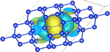
You can use the createXSF script and VESTA to visualize Wannier functions as well:
createXSF wannier.out wannier.0.xsf wannier.0.mlwf
Now the output is on a supercell rather than the unit cell. The dimensions of this supercell depend on the k-point sampling, and are 8 x 8 x 8 in this case. Use the boundary settings in VESTA to zoom in on the Wannier function, as shown above. (I used the range [0.375, 0.67].) Note that the Wannier function is centered on the Si-Si bond as expected, and has 3-fold symmetry around the bond because it is along a 111 axis. Similarly, plot the other three Wannier functions and notice that they are identical except for being centered on a bond with a different direction (four bond directions over all for the tetrahedral lattice in a diamond structure).
Next, we'll generate the band structure using the Wannier Hamiltonian output. The "mlwfH" file contains the Hamiltonian in the optimized MLWF basis. It contains an array of matrices of dimensions nCenters x nCenters (4 x 4 in this case) corresponding to the matrix elements between each of the MLWFs at one lattice site with each of the MLWFs at a nearby lattice site. The order of lattice sites is specified in the "mlwfCellMap" file. The number of lattice sites depends on the k-point sampling and fills up a Wigner-Seitz cell of the effective supercell (8 x 8 x 8 in this case). Examine wannier.mlwfCellMap, it will have a somewhat larger number of lines than 83 = 512 because it repeats boundary cells to maintain crystal symmetry. (You can visualize the cell map in gnuplot using 'splot "wannier.mlwfCellMap" u 4:5:6'.)
The above MLWF-basis Hamiltonian is a tight-binding model, but with multiple states on each lattice site (4 in this case), and connections to neighboring sites beyond just the nearest ones (as specified by the cell map). This tight-binding model reproduces the first-principles band structure from DFT exactly, and is called an ab initio tight-binding model. The following Python script calculates band structure from MLWF Hamiltonian:
#Save the following to WannierBandstruct.py:
import numpy as np
from scipy.interpolate import interp1d

#Read the MLWF cell map, weights and Hamiltonian:
cellMap = np.loadtxt("wannier.mlwfCellMap")[:,0:3].astype(np.int)
Wwannier = np.fromfile("wannier.mlwfCellWeights")
nCells = cellMap.shape[0]
nBands = int(np.sqrt(Wwannier.shape[0] / nCells))
Wwannier = Wwannier.reshape((nCells,nBands,nBands)).swapaxes(1,2)
#--- Get k-point folding from totalE.out:
for line in open('totalE.out'):
    if line.startswith('kpoint-folding'):
        kfold = np.array([int(tok) for tok in line.split()[1:4]])
kfoldProd = np.prod(kfold)
kStride = np.array([kfold[1]*kfold[2], kfold[2], 1])
#--- Read reduced Wannier Hamiltonian and expand it:
Hreduced = np.fromfile("wannier.mlwfH").reshape((kfoldProd,nBands,nBands)).swapaxes(1,2)
iReduced = np.dot(np.mod(cellMap, kfold[None,:]), kStride)
Hwannier = Wwannier * Hreduced[iReduced]

#Read the band structure k-points:
kpointsIn = np.loadtxt('bandstruct.kpoints', skiprows=2, usecols=(1,2,3))
nKin = kpointsIn.shape[0]
#--- Interpolate to a 10x finer k-point path:
xIn = np.arange(nKin)
x = 0.1*np.arange(1+10*(nKin-1)) #same range with 10x density
kpoints = interp1d(xIn, kpointsIn, axis=0)(x)
nK = kpoints.shape[0]

#Calculate band structure from MLWF Hamiltonian:
#--- Fourier transform from MLWF to k space:
Hk = np.tensordot(np.exp((2j*np.pi)*np.dot(kpoints,cellMap.T)), Hwannier, axes=1)
#--- Diagonalize:
Ek,Vk = np.linalg.eigh(Hk)
#--- Save:
np.savetxt("wannier.eigenvals", Ek)
The first two sections read in the MLWF data and set up the k-point path respectively; all the real action happens in two lines of code in the final block!
Note that the MLWF Hamitonian file format changed starting in version 1.5.0: only irreducible cells are stored in the file for compactness, and the first block of code above reads and expands the Hamiltonian to the full cell map. (See the older version of this tutorial for working with the pre-1.5.0 Wannier output.)
The Bloch Hamiltonian Hk is calculated by Fourier transforming the MLWF-basis Hamiltonian, and then we obtain the eigenvalues at each k (the band structure) by diagonalizing Hk. Run the above script "python WannierBandstruct.py", and examine the output file "wannier.eigenvals": it is a text file with the eigenvalues for each band in a column.
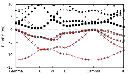
Modify the end of bandstruct.plot to compare the DFT and Wannier band structure:
#Edit end of bandstruct.plot to the following:
VBM = +0.227554  #HOMO from totalE.eigStats
eV = 1/27.2114   #in Hartrees
set xzeroaxis
set yrange [:10]
set ylabel "E - VBM [eV]"
plot for [i=1:nCols] "bandstruct.eigenvals" binary format=formatString u 0:((column(i)-VBM)/eV) every 2 w p lc rgb "black"
replot for [i=1:4] "wannier.eigenvals" u (0.1*$0):((column(i)-VBM)/eV) w l lt 1
and run "gnuplot --persist bandstruct.plot".
The Wannier band structure (plotted as lines) indeed reproduces the DFT band structure (plotted as points) exactly. Since we only constructed MLWFs from the lowest four (occupied) bands, we get the interpolated Wannier band structure only for those bands. Extending Wannier band structure interpolation to unoccupied bands and metals requires handling Entangled bands as we discuss next.