This tutorial will introduce more complicated post-processing techniques using MLWF-based ab initio tight-binding models. Here, we will calculate the frequency-dependent imaginary part of the dielectric function for aluminum, accounting for direct interband transitions.

The simplest mechanism of light absorption in materials is the direct excitation of an electron from an occupied state to an unoccupied state, absorbing one photon. Energy conservation requires that the difference between these states equals the energy of the photon. In solids, momentum conservation implies that the initial and final state are at the same k point because photons have negligible momentum at the electronic scale. Using perturbation theory and Fermi's golden rule, we can calculate the rate of this process for a given light intensity. From this rate, we can determine the corresponding imaginary part of the dielectric function as:

\[ \mathrm{Im}\epsilon(\omega) = \frac{4\pi^2 e^2}{3m_e^2\omega^2 \Omega} \int_{\mathrm{BZ}} \frac{2d\vec{k}}{V_{\mathrm{BZ}}} \sum_{n'n} (f_{\vec{k}n} - f_{\vec{k}n'}) \delta(\varepsilon_{\vec{k}n'} - \varepsilon_{\vec{k}n} - \hbar\omega) \left| \langle\vec{p}\rangle^{\vec{k}}_{n'n} \right|^2, \]

where \(\Omega\) is the unit cell volume, \(\varepsilon_{\vec{k}n}\) and \(f_{\vec{k}n}\) are Kohn-Sham eigenvalues and occupations respectively, and \(\langle\vec{p}\rangle^{\vec{k}}_{n'n}\) are the momentum matrix elements connecting band n and n' at Bloch wave-vector k. The integral averages over the Brillouin zone, and the delta function implements energy conservation. See this paper for more details; small differences here include a factor of 2 for spin degeneracy since we will use a non-relativistic calculation, and an average over spatial directions for an isotropic material that yields the factor of 3 in the denominator.

In the previous tutorial, we generated an ab initio tight-binding Hamiltonian for aluminum, which allows us to calculate the Kohn-Sham eigenvalues at arbitrary k. The occupation factors are 1 for eigenvalues smaller than mu, and 0 for those above mu. (The intermediate occupations for eigenvalues within k_BT of mu contribute negligibly for optical properties.) We also output the momentum matrix elements using the saveMomenta option of the wannier command. We will now use these outputs to calculate ImEps for aluminum:

#Save the following to WannierImEps.py:
import numpy as np

#Read the MLWF cell map, weights and Hamiltonian:    
cellMap = np.loadtxt("wannier.mlwfCellMap")[:,0:3].astype(np.int)
Wwannier = np.fromfile("wannier.mlwfCellWeights")
nCells = cellMap.shape[0]
nBands = int(np.sqrt(Wwannier.shape[0] / nCells))
Wwannier = Wwannier.reshape((nCells,nBands,nBands)).swapaxes(1,2)
#--- Get k-point folding from totalE.out:
for line in open('totalE.out'):
    if line.startswith('kpoint-folding'):
        kfold = np.array([int(tok) for tok in line.split()[1:4]])
kfoldProd = np.prod(kfold)
kStride = np.array([kfold[1]*kfold[2], kfold[2], 1])
#--- Read reduced Wannier Hamiltonian, momenta and expand them:
Hreduced = np.fromfile("wannier.mlwfH").reshape((kfoldProd,nBands,nBands)).swapaxes(1,2)
Preduced = np.fromfile("wannier.mlwfP").reshape((kfoldProd,3,nBands,nBands)).swapaxes(2,3)
iReduced = np.dot(np.mod(cellMap, kfold[None,:]), kStride)
Hwannier = Wwannier * Hreduced[iReduced]
Pwannier = Wwannier[:,None] * Preduced[iReduced]

#Constants / calculation parameters:
mu = 0.399     #in Hartrees
eV = 1/27.2114 #in Hartrees
omegaMax = 6*eV #maximum photon energy to consider
Angstrom = 1/0.5291772 #in bohrs
aCubic = 4.05*Angstrom #in bohrs
Omega = (aCubic**3)/4  #cell volume

#Calculate ImEps by Monte-Carlo sampling of the BZ integral:
nBlocks = 100  #number of blocks
nK = 1000      #number of k per block
prefactor = 8*(np.pi**2)/(3.*Omega*nK*nBlocks) #Note me=e=hbar=1 in atomic units
omegaAll = []  #Frequencies of transitions
weightAll = [] #Corresponding weights
for iBlock in range(nBlocks):
    kpoints = np.random.rand(nK,3)         #Generate random k
    Hk = np.tensordot(np.exp((2j*np.pi)*np.dot(kpoints,cellMap.T)), Hwannier, axes=1)
    Pk = np.tensordot(np.exp((2j*np.pi)*np.dot(kpoints,cellMap.T)), Pwannier, axes=1)
    Ek,Vk = np.linalg.eigh(Hk)             #Diagonalize

    Pk = np.einsum("kba,kpbc,kcd->kpad",   #Sum using Einstein notation for
        Vk.conjugate(), Pk, Vk)            #transforming Pk to eigenbasis

    #Vectorized loop over pairs of states:
    Ei = np.repeat(Ek[:,:,np.newaxis], nBands, axis=2).flatten() #Initial energy
    Ef = np.repeat(Ek[:,np.newaxis,:], nBands, axis=1).flatten()   #Final energy
    omega = Ef - Ei                                           #Energy difference
    Psq = np.sum(np.abs(Pk)**2, axis=1).flatten()        #Matrix element squared

    sel = np.where(  #Select valid transitions:
        (Ei < mu) &        #initial state occupied
        (Ef > mu) &        #final state unoccupied
        (omega < omegaMax) #energy difference in range
    )[0]
    omegaAll.append(omega[sel])
    weightAll.append(prefactor * Psq[sel] / (omega[sel]**2))
    print("Block", iBlock+1, "of", nBlocks) #Report progress

#Histogram:
nBins = 200
omegaAll = np.concatenate(omegaAll)
weightAll = np.concatenate(weightAll)
hist,binEdges = np.histogram(omegaAll, nBins, weights=weightAll, density=True)
hist *= np.sum(weightAll)  #Integral should be sum(weights), but np.histogram normalizes to 1
bins = 0.5*(binEdges[1:]+binEdges[:-1])  #bin centers
#--- Save:
outData = np.vstack((bins/eV,hist)).T #Put together in columns, converting omega to eV
np.savetxt("wannier.ImEps", outData)

The overall structure is quite similar to WannierDOS.py from the previous tutorial. In addition to the Hamiltonian, now we also transform the momentum matrix elements, first from MLWF to k space, and then to the Kohn-Sham eigenbasis. Then the code considers pairs of states at each k-point and finds transitions that contribute to light absorption at relevant frequencies. Finally, these transitions are histogrammed by frequency, appropriately weighted by the matrix elements, to calculate ImEps as a function of frequency.

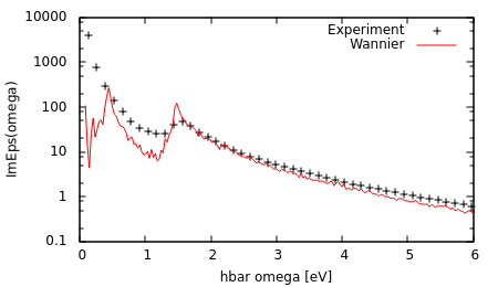
Run "python WannierImEps.py" and plot the results saved to wannier.ImEps.

Note the excellent agreement with experimental results (from ellipsometry measurements; Palik handbook) for high frequencies. At low frequencies, the experimental measurements are larger because they also include contributions due to intraband transitions. Additionally, the peak at 1.5 eV is sharper in theory than experiment because we did not account for carrier broadening effects. Accounting for these additional mechanisms and broadening effects results in much better agreement with experiment as shown here.