 |
JDFTx
1.7.0
|


|
|
JDFTx
1.7.0
|
|
| 
|
Here, we generalize from insulators and semiconductors where it is possible to single out sets of bands separated in energy from the rest, to the more general case where the bands of interest are mixed in with other bands. This is relevant not only for metals, but also for semiconductors, when we are interested in representing the unoccupied states. Specifically, this tutorial constructs maximally-localized Wannier functions (MLWFs) for aluminum, and demonstrates accurate density-of-states calculations using Monte Carlo sampling.
As before, we start with total-energy and band structure calculations. Aluminum is a face-centered cubic metal with a cubic lattice constant of 4.05 Angstroms (7.65 bohrs). We will use a norm-conserving pseudopotential for aluminum because we will use a feature (dipole matrix elements) not supported for ultrasoft pseudopotentials in the next tutorial (which builds on this tutorial).
#Save the following to common.in:
lattice face-centered Cubic 7.65
ion-species SG15/$ID_ONCV_PBE.upf
elec-cutoff 30
ion Al 0.00 0.00 0.00  0

#Save the following to totalE.in:
include common.in
kpoint-folding 12 12 12
elec-n-bands 16
elec-smearing Fermi 0.01
electronic-SCF
converge-empty-states yes
dump-name totalE.$VAR
dump End State BandEigs ElecDensity
density-of-states Total
Run the total energy calculation "mpirun -n 4 jdftx -i totalE.in | tee totalE.out". Next, follow the Band structure calculations tutorial to generate a k-point path, calculate the band structure and plot it. Specify 16 bands in the band structure calculation as well. Since this is a metal, reference the energies to mu rather than the VBM. Also note that this pseudopotential includes core electrons, so set a lower energy bound in the plots to filter these out and focus on the valence electrons.
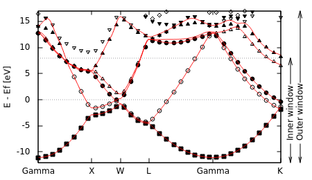
We would like Wannier functions that capture the band structure of aluminum for a few eV surrounding the Fermi level, which is the relevant range for optical properties of the metal, for example. However note that there are no sets of bands that cover this range, but are completely separated in energy from all other bands. We will therefore adopt an alternate strategy: we will require that the Wannier functions capture the band structure within a range of energies called the inner window exactly, but we will include bands from a larger range of energies called the outer window in the optimization procedure.
Specifically, let us work with 5 Wannier functions this time. In the band structure above, note that 5 bands can take us from the bottom of the valence bands approximately 11 eV below the Fermi level to just more than 9 eV above the Fermi level, where the sixth band starts (at the X point). Therefore we will set our inner window from 12 eV below the Fermi level (to include the bottom completely) to 8 eV above, which corresponds to the eigenvalue range [-0.042,0.693] Hartrees. This includes mu = 0.399 Hartrees; the ranges in the input file are absolute and not relative to mu. For the outer window, we need to pick a range that contains at least five bands throughout the Brillouin zone: we can start at the same lower end as the inner window and extend to 17 eV above the Fermi level to satisfy this, which corresponds to the eigenvalue range [-0.042,1.024] Hartrees.
With these parameters we can set up the Wannier input file:
include totalE.in

wannier \
    innerWindow -0.042 0.693 \
    outerWindow -0.042 1.024 \
    saveMomenta yes

wannier-center Gaussian -0.101403   0.435547   0.487558
wannier-center Gaussian -0.443339   0.055289  -0.446398
wannier-center Gaussian -0.361538  -0.010718   0.032397
wannier-center Gaussian -0.296948   0.326939  -0.400117
wannier-center Gaussian  0.030459  -0.158043  -0.194850

wannier-initial-state totalE.$VAR
wannier-dump-name wannier.$VAR

wannier-minimize nIterations 300
This time we have specified five wannier-center commands with trial orbitals centered at random coordinates. Note the window specifications in the wannier command. We additionally specified saveMomenta which will cause the code to output momentum matrix elements in a file suffixed "mlwfP". (We will use that output in the next tutorial.) Starting from random trial orbitals usually requires more steps to converge, which is why we increased nIterations using wannier-minimize.
Run the MLWF optimization:
mpirun -n 4 wannier -i wannier.in | tee wannier.out
and examine wannier.out. Check the final converged center coordinates and spreads. Optionally try changing the initial random orbitals: do the converged centers change? Also try adjusting the windows: what effect does the window size have on the minimized spread? Note the constraints on the window sizes: the inner window must contain at most five bands throughout, while the outer window must contain at least five bands throughout (for five wannier-center's). Five was an arbitrary choice too: you could cover a greater energy range by including six or more wannier-center's.
Use WannierBandstruct.py and bandstruct.plot from the previous tutorial to compare the DFT and MLWF-interpolated band structures. (Remember to change the number of Wannier bands in bandstruct.plot and to reference the energies to mu instead of VBM.)
The Wannier band structure follows the DFT band structure exactly within the inner window, but deviates outside it. In fact, outside the window the Wannier bands are smoother than the DFT bands since this increases localization.
We can use the MLWF-basis Hamiltonian to calculate electronic properties accurately within the inner energy window. For example, the following script calculates the density of states:
#Save the following to WannierDOS.py:
import numpy as np

#Read the MLWF cell map, weights and Hamiltonian:
cellMap = np.loadtxt("wannier.mlwfCellMap")[:,0:3].astype(np.int)
Wwannier = np.fromfile("wannier.mlwfCellWeights")
nCells = cellMap.shape[0]
nBands = int(np.sqrt(Wwannier.shape[0] / nCells))
Wwannier = Wwannier.reshape((nCells,nBands,nBands)).swapaxes(1,2)
#--- Get k-point folding from totalE.out:
for line in open('totalE.out'):
    if line.startswith('kpoint-folding'):
        kfold = np.array([int(tok) for tok in line.split()[1:4]])
kfoldProd = np.prod(kfold)
kStride = np.array([kfold[1]*kfold[2], kfold[2], 1])
#--- Read reduced Wannier Hamiltonian and expand it:
Hreduced = np.fromfile("wannier.mlwfH").reshape((kfoldProd,nBands,nBands)).swapaxes(1,2)
iReduced = np.dot(np.mod(cellMap, kfold[None,:]), kStride)
Hwannier = Wwannier * Hreduced[iReduced]

#Calculate DOS by Monte-Carlo sampling:
nBlocks = 100  #number of blocks
nK = 1000      #number of k per block
EkAll = np.zeros((nBlocks,nK,nBands))
for iBlock in range(nBlocks):
    kpoints = np.random.rand(nK,3)          #Generate random k
    Hk = np.tensordot(np.exp((2j*np.pi)*np.dot(kpoints,cellMap.T)), Hwannier, axes=1)
    Ek,Vk = np.linalg.eigh(Hk)              #Diagonalize
    EkAll[iBlock] = Ek                      #Save energies
    print("Block", iBlock+1, "of", nBlocks) #Report progress
#--- Histogram:
nBins = 400
hist,binEdges = np.histogram(EkAll, nBins, density=True)
hist *= (2*nBands)  #Integral should be 2 nBands but np.histogram normalizes to 1
bins = 0.5*(binEdges[1:]+binEdges[:-1])  #bin centers
#--- Save:
outData = np.vstack((bins,hist)).T #Put together in columns
np.savetxt("wannier.dos", outData)
The initial setup is the same as WannierBandstruct.py, but then we calculate eigenvalues on random k-points in the Brillouin zone. We are using a total of 100000 k-points above, but split it into 100 blocks of 1000 k-points each for reducing memory usage, especially to keep the size of the dot(kpoints, cellMap.T) matrix manageable. Finally, we histogram the computed eigenvalues to get the density of states.
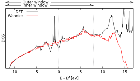
Run "python WannierDOS.py" and compare the resulting "wannier.dos" with the totalE.dos generated directly from the DFT calculation by plotting them together.
As expected, the Wannier DOS tracks the DFT one on the inner window, but not outside it. Within the inner window, notice that the Wannier DOS smooths over the spikes in the DFT DOS. Those spikes are artifacts of low-density regular k-point meshes; the Monte-Carlo sampling used 50 times as many k points and samples the Brillouin zone more evenly (no special planes / orientations), thereby avoiding these issues.
Exercise: generate Wannier functions for silicon including four unoccupied bands and generate a smooth density of states plot that beats the one in the Density of states tutorial.