This tutorial will introduce the calculation of phonon dispersion and vibrational free energies of periodic systems within JDFTx. Displacing an atom from their equilibrium positions in a molecule generates restoring forces on all atoms (within some range), which is represented by the force matrix of the system. The eigenvalues and eigenvectors of this matrix (after accounting for atom masses) represent the vibrational frequencies and normal modes of the molecule. The Free energy: Vibrations tutorial introduced the calculation of vibrational properties of molecules using the vibrations command.

In periodic systems, the force matrix has a finite range that extends beyond a single unit cell of the system. In this case, Bloch's theorem implies that the eigenvectors are waves of atom vibrations, called phonons, and the eigenvalues exhibit a band structure term the phonon dispersion. Calculating forces due to atom perturbations beyond the range of one unit cell requires performing supercell calculations and mapping the resulting properties back to the unit cell. The vibrations command within jdftx only deals with unit cell calculations and that suffices for molecules. For solids, the phonon executable handles constructing supercells, performing perturbed calculations and mapping the so-calculated phonon properties back to the original unit cell.

Let's start with the silicon calculations from the Band structure calculations tutorial (which we also used for the Separated bands Wannier tutorial). Remember to run the total energy calculation, construct the k-point path, and review the electronic band-structure calculation and plotting.

First, we set up a input file for phonon:

#Save the following to phonon.in
include totalE.in          #Full specification of the unit cell calculation
initial-state totalE.$VAR  #Start from converged unit cell state
dump-only                  #Don't reconverge unit cell state

phonon supercell 2 2 2     #Calculate force matrix in a 2x2x2 supercell

and run it with:

mpirun -n 4 phonon -i phonon.in | tee phonon.out

This may take several minutes, so run the above command and then follow along below as we examine the output generated. Once again, note that we use the executable phonon, separate from jdftx. The input file is extremely simple, relying on totalE.in for the entire specification of the unit cell calculation and the corresponding converged unit cell results (totalE.$VAR).

The only addition is the phonon command, for which the only required argument is the supercell size in which to calculate the force matrix. The supercell size must be a factor of the k-point folding: since we have 8x8x8 folding in this case, only 1, 2, 4 and 8 are acceptable for each dimension of the supercell. Note that the calculation will be substantially more expensive as the supercell size is increased.

Now examine the output in (or that is being written to) phonon.out. After listing all the commands (including default ones), the usual initialization of a unit cell calculation follows under the heading “Unit cell calculation.” This part ends on the energy evaluation in the unit cell at a fixed state (corresponding to dump-only).

Next, phonon constructs the supercell and determines its symmetries. It figures out all the atom displacements necessary to generate the force matrix: 2 atoms/cell x 3 Cartesian directions x 2 signs for central difference derivative = 12 for this example, and then finds the number of symmetry-irreducible perturbations, which happens to be just 1 in this case!

Then, for each symmetry-irreducible perturbation, it runs a supercell calculation with atom displaced (by dr = 0.01 bohrs by default, see phonon to change this) under the heading “Perturbed supercell calculation X of N.” The output format for each such calculation is also the usual JDFTx initialization followed by SCF (or ElecMinimize), but note that the lattice vectors are all twice as large, the bands and basis 8 times larger, while the k-point folding is halved, because this is a 2x2x2 supercell calculation.

At the end of each supercell calculation, phonon reports the energy and force change due to the perturbation per unit cell. Always make sure that these are one-two orders of magnitude larger than the convergence thresholds, either by adjusting those thresholds, or by adjusting dr in the phonon command.

After all the supercell calculations, phonon collects force matrix contributions from each and outputs this to the binary totalE.phononOmegaSq file (which we will use below). It also outputs the text file totalE.phononCellMap, which lists the order of neighboring unit cells for the force matrix output (in exactly the same format as the wannier.mlwfCellMap encountered in the Separated bands Wannier tutorial). Meanwhile, totalE.phononBasis lists the order of atom perturbations in the phonon force matrix. The totalE.phononHsub binary file contains electron-phonon matrix elements, which we will not discuss in this tutorial.

The code ends with a summary of the zero-point energy and vibrational free energy contributions, in exactly the same format as the output of the vibrations command, except it is now the (free-)energy contributions per unit cell of a periodic system. Note that phonon accounts for 3D periodicity for the Si example here, but will automatically switch to 2D or 1D periodicity, as appropriate, based on the geometry specified in the coulomb-interaction command.

Finally, we will calculate and plot the phonon dispersion from the force matrix output using this python script:

#Save the following to PhononDispersion.py:
import numpy as np
from scipy.interpolate import interp1d

#Read the phonon cell map and force matrix:
cellMap = np.loadtxt("totalE.phononCellMap")[:,0:3].astype(int)
forceMatrix = np.fromfile("totalE.phononOmegaSq", dtype=np.float64)
nCells = cellMap.shape[0]
nModes = int(np.sqrt(forceMatrix.shape[0] / nCells))
forceMatrix = np.reshape(forceMatrix, (nCells,nModes,nModes))

#Read the k-point path:
kpointsIn = np.loadtxt('bandstruct.kpoints', skiprows=2, usecols=(1,2,3))
nKin = kpointsIn.shape[0]
#--- Interpolate to a 10x finer k-point path:
nInterp = 10
xIn = np.arange(nKin)
x = (1./nInterp)*np.arange(1+nInterp*(nKin-1)) #same range with 10x density
kpoints = interp1d(xIn, kpointsIn, axis=0)(x)
nK = kpoints.shape[0]

#Calculate dispersion from force matrix:
#--- Fourier transform from real to k space:
forceMatrixTilde = np.tensordot(np.exp((2j*np.pi)*np.dot(kpoints,cellMap.T)), forceMatrix, axes=1)
#--- Diagonalize:
omegaSq, normalModes = np.linalg.eigh(forceMatrixTilde)

#Plot phonon dispersion:
import matplotlib.pyplot as plt
meV = 1e-3/27.2114
plt.plot(np.sqrt(omegaSq)/meV)
plt.xlim([0,nK-1])
plt.ylim([0,None])
plt.ylabel("Phonon energy [meV]")
#--- If available, extract k-point labels from bandstruct.plot:
try:
    import subprocess as sp
    kpathLabels = sp.check_output(['awk', '/set xtics/ {print}', 'bandstruct.plot']).split()
    kpathLabelText = [ label.split('"')[1] for label in kpathLabels[3:-2:2] ]
    kpathLabelPos = [ nInterp*int(pos.split(',')[0]) for pos in kpathLabels[4:-1:2] ]
    plt.xticks(kpathLabelPos, kpathLabelText)
except:
    print ('Warning: could not extract labels from bandstruct.plot')
plt.show()

Note that the overall strategy is exactly analogous to generating the electronic band structure from the Wannier Hamiltonian output. Using information from the cell map, we transform the force matrix to k space and diagonalize it to get the square of the phonon frequencies. Most of the lines of code above deal with input/output and beautifying the plot.

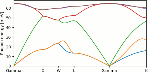
Running "python PhononDispersion.py" produces the phonon dispersion curves (or band structure) shown below and at the top of this page:

Note that the phonon energies increase linearly from zero near the Gamma point, rather than quadratically as the electron energies do in band structure plots, because the phonon energy is the square root of the diagonalized quantity. This results in finite group velocities (the sound speeds) of phonons near k=0.