While the solvation options described in the previous tutorial are sufficient to describe the solvation of molecules in fluids such as water, these fluids are not sufficient by themselves to describe the solvation of charged species like ions. A solution with charged species will necessarily contain both positive and negative ions, and the response of the liquid is critically dependent on the response of these ions. In dilute ionic solutions (electrolytes), the ions to do not strongly interact with each other or the solute / surface under consideration, beyond the mean-field electrostatic interaction. In this limit, it is appropriate to approximate the effects of ions in the solution using a linearized Poisson-Boltzmann equation (roughly equivalent to Debye-Huckel theory). This tutorial introduces solvation of charged species by calculating the dissociation constant of water, related to the equilibrium constant of the reaction 2H₂O → H₃O⁺ + OH^-.

We will need very similar calculations for three species now, H₂O, H₃O⁺ and OH^-. We can use a single set of input files for all three calculations using another neat trick in JDFTx, environment variable substitution (see Input file documentation). First, let's collect the common commands as usual in common.in:

#Save to common.in
lattice Cubic 15
coulomb-interaction Isolated
coulomb-truncation-embed 0 0 0
ion-species GBRV/$ID_pbe.uspp
elec-cutoff 20 100
coords-type cartesian

include ${CONFIG}.ionpos
initial-state ${CONFIG}.$VAR
dump-name ${CONFIG}.$VAR
dump End None

elec-initial-charge ${CHARGE}

fluid LinearPCM
pcm-variant CANDLE
fluid-solvent H2O
fluid-cation Na+ 1.
fluid-anion F- 1.

This time, we are using solvation in all calculations, so we can put all the solvation commands above. Note that in addition to the solvent, this calculation specifies 1M concentration of sodium and fluoride ions. The choice of Na+ and F- is primarily because NaF is a well-known non-adsorbing electrolyte, and this is a good reminder that ions in the continuum solvent will not specifically interact or react with your solute (beyond electrostatics). (The different ion choices in the code behave differently only for ClassicalDFT. Please stick to Na+ and F- in the continuum electrolyte to remind you of the above facts, regardless of the real electrolyte you are trying to calculate for, and consider explicit adsorption of those ions in the electronic DFT calculation if it is important.)

Additionally, note that we have not specified any one solute! Instead, we are generically including an ionpos file called ${CONFIG}.ionpos, reading state from and writing outputs to files with name pattern ${CONFIG}.$VAR. We will select ${CONFIG} at run time below. Similarly we specify ${CHARGE} at run time, indicating how many extra electrons the DFT calculation should have relative to the neutral system. (Note that the charge is measured in electrons, as nature intended, so OH^- will have charge +1 and H₃O⁺ will have charge -1.)

Now for total energy calculations including ionic-minimization, we can use the input file:

#Save the following to totalE.in
include common.in
ionic-minimize nIterations 10
dump End State BoundCharge

and for vibrations (which we need for the free energy):

#Save the following to vibrations.in
include common.in
vibrations \
    centralDiff yes \
    translationSym yes \
    rotationSym yes

Next, we need initial ionic positions for all three calculations:

#Save the following to H2O.ionpos
ion O   0.00 0.00  0.00  0
ion H   0.00 1.13 +1.45  1
ion H   0.00 1.13 -1.45  1

,

#Save the following to H3O+.ionpos
ion O   0.00  0.00  0.00  0
ion H   1.81 -0.25 -0.25  1
ion H  -0.25  1.81 -0.25  1
ion H  -0.25 -0.25  1.81  1

and

#Save the following to OH-.ionpos
ion O   0.00 0.00 0.00  0
ion H   0.00 0.00 1.84  1

These have all been set up to represent initial O-H bond lengths of 0.97 Angstroms and H-O-H bond angles of 104.5 degrees. The orientation is chosen to maximize symmetries in a cubic unit cell (check the symmetries output at the start of the initialization); this is not necessary, but it is good practice that helps reduce the number of steps in geometry optimization.

Finally, let's write a script that runs everything for one system:

#!/bin/bash
export CONFIG="$1"
export CHARGE="$2"
jdftx -i totalE.in | tee $CONFIG-totalE.out
jdftx -i vibrations.in | tee $CONFIG-vibrations.out

Save the above to run.sh, and do "chmod +x run.sh" to make it executable. This script reads the configuration name and charge as input parameters, sets them to named environment variables CONFIG and CHARGE, which jdftx then uses to substitute in the input files created above.

Using this script, we can run all the necessary calculations as:

./run.sh H2O   0
./run.sh H3O+ -1
./run.sh OH-  +1

After running for a while, this will generate six output files, energy minimization and vibration analysis for the three configurations. Examine the output files: everything should look familiar by now. Since we didn't initialize the solvated calculation from a vacuum one, the code runs an initial minimization in vacuum to get sane wavefunctions and electron density, before turning on the solvent. Note how the energy difference between the initial vacuum calculation and the first solvated calculation (this is reported as the single-point solvation energy estimate at the end of the first electronic minimize with solvation) is an order of magnitude larger for the two charged species compared to the neutral one.

The fluid screening lines now additionally report an ionic screening length. Note that this time we also calculated vibrational frequencies in solution. Examine the frequencies and reported normal modes of vibration: do they all line up with intuition regarding the symmetries of the molecules/ions?

Here follow the total (solvated) energies and vibrational free energies of the species, with the last line representing the difference for the reaction 2H₂O → H₃O⁺ + OH^-, all in Hartrees:

Configuration	Etot	Avib	A (free energy)
H2O	-17.28095	0.02076	-17.26019
H3O+	-17.70547	0.03305	-17.67242
OH-	-16.81064	0.00871	-16.80193
Reaction	0.04579	0.00024	0.04603

Notice that the vibrational contribution almost cancels out in the difference, because the reactants and the products all have the same number of O-H bonds of comparable stiffness. This will not be true in general though, and vibration calculations are usually necessary for reliable free energies.

The reaction free energy, DeltaA, calculated above sets the equilibrium:

$ exp(\frac{-\triangle A}{kT}) = \frac{[H3O+][OH-]}{[H2O]^2} $

Using its definition, the dissociation constant of water is therefore:

$ pK_w = -log_{10}([H3O+][OH-]) = \frac{\triangle A}{2.303 kT} - 2 log_{10}[H2O] $

With kT = 0.000944 Hartrees and [H2O] = 55.5M at standard temperature and pressure, CANDLE therefore predicts pKw = 17.7 in reasonable agreement with the well-known experimental value pKw = 14.

In contrast, rerunning all the above calculations with the GLSSA13 LinearPCM (what all would you change in the input file?), which once again is identical to VASPsol and vey similar to SCCS, we get the results:

Configuration	Etot	Avib	A (free energy)
H2O	-17.27957	0.02082	-17.25875
H3O+	-17.70966	0.03218	-17.67748
OH-	-16.76710	0.00866	-16.75844
Reaction	0.08238	-0.00080	0.08158

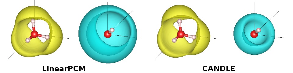
which predicts a pKw = 34.0 that is rather inaccurate. Looking at the energies, note that the one which differs the most from CANDLE is OH-. A very important feature in CANDLE is that it correctly handles the difference in solvation between cations and anions of the same size (CA expands to Charge-Asymmetric). This is why it can describe both OH- and H3O+ correctly with the same parametrization, in contrast to previous solvation models like GLSSA13/VASPsol/SCCS that require separate parametrizations.

This is also noticeable in the bound charge distributions, visualized using createXSF and VESTA as before. Note the similarity between CANDLE and LinearPCM(GLSSA13) for H3O+ (and also for H2O in the previous tutorial), while CANDLE places the bound charge closer to OH- than LinearPCM.