The previous tutorial introduced phonon dispersion calculations using the example of silicon using a small 2x2x2 supercell. Realistic phonon calculations typically require at least 4x4x4 supercells for bulk 3D materials, and 6x6x1 supercells for 2D materials like graphene. Large supercells quickly make phonon calculations extremely expensive. This tutorial shows how to split a phonon calculation into smaller chunks, which can be efficiently run in parallel.

Let's start with the graphene calculations from the Two-dimensional materials tutorial. First, we need to make sure the unit cell calculation saves its state:

#Save the following to totalE.in:
include common.in
kpoint-folding 12 12 1
elec-smearing Fermi 0.01
dump-name totalE.$VAR
dump End ElecDensity State

which can be run with "mpirun -n 4 jdftx -i totalE.in | tee totalE.out". Also make sure that the k-point paths and plot script for band structure have been generated as described in the Two-dimensional materials tutorial.

Now, set up the phonon input file, admittedly still with an inadequately small supercell size, to facilitate a quick test:

#Save the following to phonon.in:
include totalE.in
initial-state totalE.$VAR
dump-only

phonon supercell 2 2 1 ${phononParams}

We will replace phononParams using environment variables to run the phonon code in various modes; alternatively, you could create separate input files for each stage.

First, perform a phonon dry run using:

phonon -ni phonon.in

and examine the output. The output is very similar to the previous tutorial, except that in the dry run, electronic optimizations and file outputs are skipped. Additionally, at the end, the code reports a summary of the supercell calculations necessary:

Parameter summary for supercell calculations:
    Perturbation: 1  nStates: 7
    Perturbation: 2  nStates: 20
Use option iPerturbation of command phonon to run each supercell calculation separately.

This time there are two symmetry-irreducible perturbations (C atom displaced in plane, and out of plane) which have different symmetries and hence different numbers of reduced k points (nStates).

Now, we can run the two supercell calculations separately using:

export phononParams="iPerturbation 1"
mpirun -n 4 phonon -i phonon.in | tee phonon.1.out

and

export phononParams="iPerturbation 2"
mpirun -n 4 phonon -i phonon.in | tee phonon.2.out

I used 4 processes here for the four cores in my laptop. If running on a compute cluster, it would instead make sense to run the first calculation with 7 processes and the second with 20 (or 10 or 5) in order to get best parallel efficiency. Additionally, the two calculations can be launched on separate (sets of) nodes concurrently.

Examine the two output files. Each runs only one of the two supercell calculations and saves the corresponding outputs (eg. totalE.phonon.1.dforces), but does not output the cell map, force matrix or free energies.

Finally, run:

export phononParams="collectPerturbations"
mpirun -n 4 phonon -i phonon.in | tee phonon.out

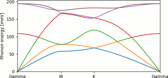
which reads the output from the previous calculations, puts it all together and outputs the cell map, force matrix and free energies. Using the python script from the previous tutorial produces the phonon dispersion shown at the top of the page.

Exercise: using a compute cluster, run the realistic 6x6x1 supercell version, making sure to pick the optimum parallelization for each supercell calculation, based on the dry run summary (and the hardware configuration of your cluster). How do the results compare with the quick test here?