The previous sections introduced two classes of geometries specified using the coulomb-interaction command: isolated systems like molecules which are non-periodic in all three directions, and crystalline solids which are periodic in all three directions. This section explores systems which are periodic in two directions and non-periodic in one direction, which is specified using

coulomb-interaction Slab 001

where the second parameter specifies which direction is periodic. (Similarly, "coulomb-interaction Wire 001" specifies a geometry which is periodic only along the third direction, which is useful for systems such as nanowires, nanotubes and DNA.)

The slab geometry, as the name suggests, is useful for treating slabs of material surrounded by empty space or solvent on two sides, which in turn is usually meant to describe the properties of the surface of a solid (solid-vacuum interface) or a solid-liquid interface.

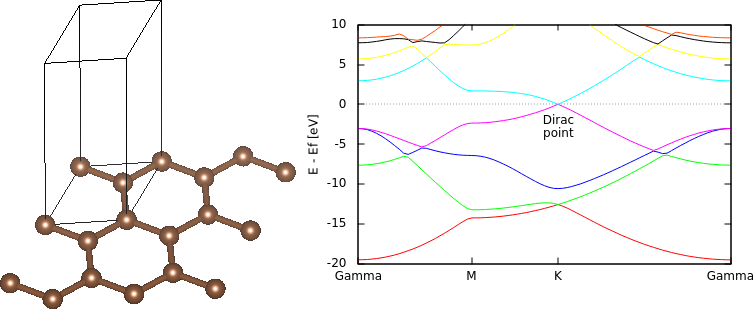
First, we'll take an extreme example which is all surface: graphene. We will setup the geometry by peeling out a single layer of graphite from the Dispersion (vdW) corrections tutorial:

#Save the following to common.in:
coulomb-interaction Slab 001
coulomb-truncation-embed 0 0 0
lattice Hexagonal 4.651 15           #Exact vertical dimension no longer matters

ion C  0.000000  0.000000  0.0   0
ion C  0.333333 -0.333333  0.0   0

ion-species GBRV/$ID_pbe.uspp
elec-cutoff 20 100

We will then perform total energy and band structure calculations as usual using the input files:

#Save the following to totalE.in:
include common.in
kpoint-folding 12 12 1               #Need k-points only in periodic directions
elec-smearing Fermi 0.01
dump-name totalE.$VAR
dump End ElecDensity


#Save the following to bandstruct.in:
include common.in
include bandstruct.kpoints
fix-electron-density totalE.$VAR
elec-n-bands 8
dump-name bandstruct.$VAR
dump End BandEigs


#Save the following to bandstruct.kpoints.in:
kpoint 0.00000  0.00000  0.0     Gamma
kpoint 0.50000  0.00000  0.0     M
kpoint 0.66667 -0.33333  0.0     K
kpoint 0.00000  0.00000  0.0     Gamma

and the commands:

bandstructKpoints bandstruct.kpoints.in 0.02 bandstruct  #Generate bandstruct.kpoints and bandstruct.plot
mpirun -n 4 jdftx -i totalE.in | tee totalE.out          #Run total energy calculation
mpirun -n 4 jdftx -i bandstruct.in                       #Run bandstructure calculation
gnuplot --persist bandstruct.plot                        #Plot band structure

Edit the bandstructure plot to reference the enegies against the Fermi level (mu from final FillingsUpdate line) and convert it to eV, to get the band structure shown above. Note the Dirac point seen at the K point as the intersection of two bands exactly at the Fermi level.

Next, examine the effect of the Coulomb truncation on the energy levels of the system. For a neutral slab (or 2D material) in vacuum, the electrostatic potential exponentially decays away from the surface(s). With Coulomb truncation in Slab mode, this property is reproduced even in the plane-wave basis, whereas without it, the potential has an undetermined offset as in the 3D periodic (bulk solid) case. Repeat the total-energy calculation above for increasing lengths of the unit cell, both with and without the two Coulomb truncation lines, and note the final mu in each case. (This could be easily automated using variable substitution as in the Setting up molecule geometries tutorial.)

This mu is the chemical potential or Fermi level of electrons relative to zero potential at infinity, and therefore corresponds to the work function of the material. For graphene, testing the convergence of mu (in Hartrees) with respect to cell length Lz (in bohrs) yields:

Lz	mu with truncation	mu without truncation
15	-0.155825	+0.019651
20	-0.156102	-0.024394
25	-0.156106	-0.050738
30	-0.156103	-0.068295

As expected, mu converges exponentially with cell size with truncation, but very slowly (with an error inversely proportional to cell volume) without truncation.