Our examples of periodic materials have so far dealt with perfect crystals. Defects in crystals that break this periodicity play a critical role in the behavior of real materials for several properties. DFT calculations approximate defects in a supercell containing several unit cells of the material, with the defect introduced in just one of those unit cells. This requires care to ensure that the interaction of defects with its periodic images (on the superlattice) is negligible, especially when the defect is charged.

Bulk calculation

We will introduce defect calculation techniques in JDFTx here using the example of a nitrogen atom substituting a carbon atom (denoted N_C) in diamond. First, we need to perform calculation of a perfect 'bulk' diamond crystal, which has a face-centered cubic lattice with a 2 atom basis:

#Save the following to bulk.in
lattice face-centered Cubic 6.74

ion C 0.00 0.00 0.00 1
ion C 0.25 0.25 0.25 1

ion-species GBRV/$ID_pbe.uspp
elec-cutoff 20 100

kpoint-folding 4 4 4
elec-smearing Fermi 0.01

electronic-SCF
converge-empty-states yes
dump End EigStats

Run jdftx on bulk.in to get the total energy and the eigenvalue statistics for the perfect crystal. We will particularly require the HOMO (VBM) and LUMO (CBM) energies from the bulk.eigStats output.

This bulk structure will also serve as the reference state for determining the chemical potential of carbon atoms (bulk diamond will be the carbon reservoir for the defect). For the nitrogen atom, we need the energy of the reference state, a nitrogen molecule, calculated using the same pseudopotentials:

#Save the following to N2.in
lattice face-centered Cubic 20.
coulomb-interaction Isolated
coulomb-truncation-embed 0 0 0

coords-type Cartesian
ion N 0. 0. +1.03 1
ion N 0. 0. -1.03 1

ion-species GBRV/$ID_pbe.uspp
elec-cutoff 20 100

electronic-SCF
ionic-minimize nIterations 10
dump End None

Run jdftx on N2.in to get the total energy of an N₂ molecule.

Perfect supercell

Next, we need to construct a perfect supercell of the diamond crystal. Here, we will make a 2x2x2 supercell of the primitive unit cell calculated above. To do this, we will scale up the lattice vectors by a factor of 2 using latt-scale. We will correspondingly reduce the kpoint-folding by a factor of 2, so that the effective supercell sampled by the k-mesh remains the same as the unit cell calculation. We will also need to repeat the atoms to account for all the unit cells within the supercell. The net result of this is scaling down the lattice coordinates of the two atoms in the unit cell by a factor of 2 (since the lattice vectors have doubled), and then repeating them by adding all combinations of 0 and 1/2 in each of the three coordinates to fill up eight unit cells within the 2x2x2 supercell. (Note that this amounts to the transformation detailed in Pt(100) setup with matrix M = 2 x identity.) The resulting input file for the perfect supercell is:

#Save the following to supercell.in
lattice face-centered Cubic 6.74
latt-scale 2 2 2

ion C 0.000 0.000 0.000 1
ion C 0.125 0.125 0.125 1
ion C 0.000 0.000 0.500 1
ion C 0.125 0.125 0.625 1
ion C 0.000 0.500 0.000 1
ion C 0.125 0.625 0.125 1
ion C 0.000 0.500 0.500 1
ion C 0.125 0.625 0.625 1
ion C 0.500 0.000 0.000 1
ion C 0.625 0.125 0.125 1
ion C 0.500 0.000 0.500 1
ion C 0.625 0.125 0.625 1
ion C 0.500 0.500 0.000 1
ion C 0.625 0.625 0.125 1
ion C 0.500 0.500 0.500 1
ion C 0.625 0.625 0.625 1

ion-species GBRV/$ID_pbe.uspp
elec-cutoff 20 100

kpoint-folding 2 2 2
elec-smearing Fermi 0.01

electronic-SCF
converge-empty-states yes
dump End EigStats ElecDensity Dtot

Run jdftx on supercell.in to get the energy, eigStats, electron density and electrostatic potential of the perfect supercell. Notice that the band edges (HOMO and LUMO) are identical within numerical error, and the total energy is exactly 8 times that of the bulk unit cell, as expected.

Neutral defect

Now, let us substitute one of the carbon atoms with nitrogen, say the one at the origin without loss of generality. This gives us the input for the neutral N_C defect:

#Save the following to N_C-0.in
lattice face-centered Cubic 6.74
latt-scale 2 2 2

ion N 0.000 0.000 0.000 1  #Note C replaced by N
ion C 0.125 0.125 0.125 1
ion C 0.000 0.000 0.500 1
ion C 0.125 0.125 0.625 1
ion C 0.000 0.500 0.000 1
ion C 0.125 0.625 0.125 1
ion C 0.000 0.500 0.500 1
ion C 0.125 0.625 0.625 1
ion C 0.500 0.000 0.000 1
ion C 0.625 0.125 0.125 1
ion C 0.500 0.000 0.500 1
ion C 0.625 0.125 0.625 1
ion C 0.500 0.500 0.000 1
ion C 0.625 0.625 0.125 1
ion C 0.500 0.500 0.500 1
ion C 0.625 0.625 0.625 1

ion-species GBRV/$ID_pbe.uspp
elec-cutoff 20 100

kpoint-folding 2 2 2
elec-smearing Fermi 0.01

electronic-SCF
converge-empty-states yes
dump End Dtot ElecDensity

After running jdftx on N_C-0.in, we will get the total energy of the neutral defect (in addition to the electrostatic potential and density which we will use below). From this, we can compute the formation energy of the neutral defect as

\[ E_{\text{form}}^{(0)} = E(\text{N_C-0}) - E(\text{supercell}) - (\mu_N - \mu_C), \]

where \( E(\text{N_C-0}) \) and \( E(\text{supercell}) \) are the total energies (F) obtained from the N_C-0.in and supercell.in calculation output files respectively. Above, \( \mu_C \) is the chemical potential of the carbon atom, equal to the energy per atom in the reference state for carbon, which is just perfect diamond in this case. Therefore, \( \mu_C = E(\text{bulk})/2 \) from the unit cell calculation above. Similarly, \( \mu_N = E(\text{N2})/2 \) from the nitrogen molecule calculation above. This results in a formation energy of approximately 4.0 eV for the neutral defect.

Exercise: converge the formation energy of the neutral N_C defect with respect to supercell size by performing 3x3x3 and 4x4x4 supercell calculations. (These will of course be much slower than the 2x2x2 calculation above.)

Charged defects

Let us now compute the energy of the N_C defect with one fewer or one extra electron i.e. in the +1 or -1 charge states respectively. Unlike the previous case, we cannot just take the energy of the supercell calculation to compute the formation energy because charged defects will interact very strongly with their periodic images due by the long-range 1/r Coulomb interaction. Consequently, we correct the energy of a defect with charge q by comparing the energy and electrostatic potential of a Gaussian charge distribution embedded in a uniform medium with the dielectric constant of our bulk material, each computed with isolated and periodic boundary conditions. This yields an energy correction [9]

\[ E_{\text{corr}} = E_{\text{isolated}} - E_{\text{periodic}} + qV, \]

which we should add to the total energy in the DFT calculation. The last term is an alignment contribution accounting for the difference in the electrostatic potential of the model charge far from the defect, compared to that calculated by DFT.

JDFTx implements this correction scheme controlled by charged-defect-correction and directly reports the net correction energy including all these terms (See [33] for implementation details.) Run jdftx on input files for the negative defect (one extra electron):

#Save the following to N_C-1.in
include N_C-0.in

elec-initial-charge +1                 #One extra electron
charged-defect 0.00 0.00 0.00  +1  1   #Gaussian charge model
charged-defect-correction \
    supercell.d_tot \   #reference potential for alignment
    5.8    \            #bulk dielectric constant
    4. \                #cutoff distance for alignment potential
    1.                  #smoothness in alignment potential cutoff

and the positive defect (one less electron):

#Save the following to N_C+1.in
include N_C-0.in

elec-initial-charge -1                 #One less electron
charged-defect 0.00 0.00 0.00  -1  1   #Gaussian charge model
charged-defect-correction \
    supercell.d_tot \   #reference potential for alignment
    5.8    \            #bulk dielectric constant
    4. \                #cutoff distance for alignment potential
    1.                  #smoothness in alignment potential cutoff

to get the total energy (F) from the corresponding output files, and the net energy correction reported at the end of each output file. In addition to setting the charge of the system using elec-initial-charge, these input files specify a Gaussian model charge using charged-defect and parameters for the correction scheme using charged-defect-correction. The correction reads in the electrostatic potential of the perfect supercell as a reference and takes the bulk dielectric constant of the material as an input. Note that this dielectric constant must be the static value \( \epsilon_0 \) if atoms are relaxed self-consistently (skipped here for simplicity), but the high-frequency value \( \epsilon_\infty \) if the atoms are held fixed. For diamond, \( \epsilon_0 \approx \epsilon_\infty \) in any case.

The final two parameters of charged-defect-correction specify the region of space used for determining the alignment offset between the DFT calculation and the model problem: the average is performed outside a cutoff radius with a smooth transition. The cutoff radius should exclude the location of the defect and neighboring atoms, but be smaller than the radius of the Wigner-Seitz unit cell of the superlattice.

Using the corrected energies of the charged supercells \( E(\text{N_C-}q) \), for q=+1 and -1, we can compute the formation energies of each charge state as:

\[ E_{\text{form}}^{(q)} = E(\text{N_C-}q) - E(\text{supercell}) - (\mu_N - \mu_C - q\mu), \]

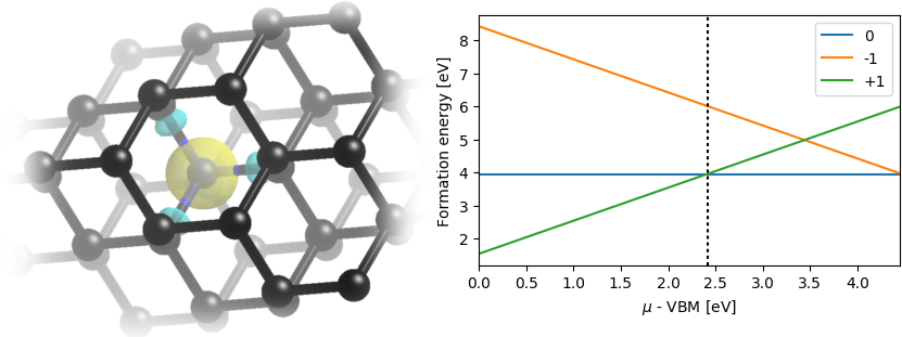
where the last term accounts for the different numbers of electrons based on the electron chemical potential \( \mu \). Therefore, the formation energies of the charged defect will depend on the position of the Fermi level, which in a semiconductor will depend on the net doping. We will therefore plot the formation energies as a function of the Fermi level, typically spanning the range from VBM (HOMO) to CBM (LUMO).

The following python script uses the energies from all the calculations above to plot the formation energies of the neutral and both charged defects:

import numpy as np
import matplotlib.pyplot as plt

#Bulk properties:
muC = -11.408263/2 #energy per carbon atom in bulk
muN = -19.962539/2 #energy per N atom in N2 molecule
HOMO = 0.491719
LUMO = 0.655073

#Supercell properties:
Esup  = -91.266105 #energy of perfect supercell
EN_C0 = -95.397922 #energy of neutral N_C defect
EN_CM = -94.758574+0.016575 #energy of -1 N_C defect (including correction)
EN_CP = -96.009777+0.031387 #energy of +1 N_C defect (including correction)

#Compute defect formation energies:
mu = np.linspace(HOMO, LUMO) #range of electron chemical potentials
EfN_C0 = EN_C0 - Esup - (muN - muC - mu*( 0)) #neutral formation energy
EfN_CM = EN_CM - Esup - (muN - muC - mu*(-1)) #-1 formation energy
EfN_CP = EN_CP - Esup - (muN - muC - mu*(+1)) #+1 formation energy
CTL_M = EN_CM - EN_C0  #-1|0 charge transition level
CTL_P = EN_C0 - EN_CP  #0|+1 charge transition level relative to VBM

#Report and plot charge transition levels:
eV = 1/27.2114
print('Ef(0):', EfN_C0[0]/eV, 'eV')
print('CTL -1|0:', (CTL_M-HOMO)/eV, 'eV wrt VBM')
print('CTL 0|+1:', (CTL_P-HOMO)/eV, 'eV wrt VBM')
plt.figure(1, figsize=(5,3))
plt.plot((mu-HOMO)/eV, EfN_C0/eV, label='0')
plt.plot((mu-HOMO)/eV, EfN_CM/eV, label='-1')
plt.plot((mu-HOMO)/eV, EfN_CP/eV, label='+1')
plt.axvline((CTL_M-HOMO)/eV, color='k', ls='dotted')
plt.axvline((CTL_P-HOMO)/eV, color='k', ls='dotted')
plt.xlim(0., (LUMO-HOMO)/eV)
plt.xlabel(r'$\mu$ - VBM [eV]')
plt.ylabel('Formation energy [eV]')
plt.legend()
plt.savefig('CTL.png', bbox_inches='tight')
plt.show()

Note that at each value of \( \mu \), a particular charge state will have the lowest energy and be the most stable configuration in equilibrium. The \( \mu \) values at which the charge state changes, given by the intersection of the lines corresponding to two adjacent charge states, are called the charge transition levels. In the present case, we find that the -1 to 0 transition occurs 4.5 eV above the HOMO: this is the acceptor energy level with an ionization energy of 4.5 eV. The 0 to +1 transition is 2.4 eV above the HOMO: this is the donor energy level with an ionization energy (relative to the LUMO) of 2.0 eV.

Exercise: converge the charged defect results with supercell size. Plot the results as a function of supercell size with and without the correction. How big of a supercell would you need for 0.1 eV accuracy with and without the correction?

Exercise: use createXSF and VESTA to plot the charge distribution of the defect, the difference between electron density in the charged defect and the perfect supercell, as shown below.

Exercise: calculate the charge transition levels of B and P substitutions of Si atoms in silicon, and identify the donor and acceptor level ionization energies for each.