Now we move on from a ferromagnetic metal to an antiferromagnetic insulator, ferrous oxide (FeO). This tutorial introduces DFT + U, a technique to compensate for errors in density-functional theory for localized electrons (such as d and f electrons).

Ferrous oxide has a rock-salt structure which consists of two inter-penetrating face-centered cubic lattices of iron and oxygen atoms, with cubic lattice contant 4.32 Angstroms (8.16 bohrs) each. We could set up that geometry using:

lattice face-centered Cubic 8.16
ion Fe 0.0 0.0 0.0  0
ion O  0.5 0.5 0.5  0

However, that geometry contains only one Fe atom per unit cell, which would then constrain every Fe atom in our structure to have the same magnetic moment, resulting in a ferromagnetic structure. We need a minimum of two Fe atoms in the unit cell to obtain an antiferromagnetic structure, so we could construct one possible antiferromagnetic structure by doubling up the unit cell:

#Save the following to FeO.in:
lattice face-centered Cubic 8.16
latt-scale 1 1 2.01             #Slightly break symmetry
kpoint-folding 6 6 3

ion Fe 0.0 0.0 0.00  0
ion Fe 0.0 0.0 0.50  0
ion O  0.5 0.5 0.25  0
ion O  0.5 0.5 0.75  0

ion-species GBRV/$ID_pbe.uspp
elec-cutoff 20 100
elec-smearing Fermi 0.01
electronic-SCF

spintype z-spin
initial-magnetic-moments Fe +5 -5

dump End None
density-of-states Total
dump-name PBE.$VAR

Note that we used latt-scale to double the last lattice vector. Once we make the system antiferromagnetic, we will break the rotational symmetry between the first two and the third lattice directions. We make the third direction sightly different from exactly twice as long so that the system does not get constrained artifically by symmetries; in real calculations we would then optimize the lattice to find the equilibrium geometry and distortions (if any), but I skip it above to make the calculations quicker. Note that we correspondingly halved the last fractional coordinate of each atom, and repeated them once with an offset of 0.5 along the last direction. We also reduced the kpoint folding by half along that direction, since the unit cell is longer to start with in that direction.

The remaining setup is similar to the iron calculation in the Magnetism tutorial, except that instead of specifying a guess for the total magnetization of the unit cell using elec-initial-magnetization (which would be zero for an antiferromagnet), we specify guesses for each Fe atom individually using initial-magnetic-moments. Specifically, we set the initial magnetization to be equal and opposite for the two atoms in the unit cell.

Run this calculation as usual using:

mpirun -n 4 jdftx -i FeO.in | tee PBE.out

and examine the output file. This time, the FillingsUpdate lines report a total magnetization close to zero, but an absolute magnetization far from zero due to the equal and opposite magnetic moments. Additionally the absolute magnetization is 7.1, which lines up well with the absolute sum of per-atom magnetic moments estimated in the Lowdin analysis, +3.5 and -3.5. (Note that these need not line up exactly; per-atom magnetic moments do not have an unambiguous physical definition, and Lowdin analysis only provides estimates.)

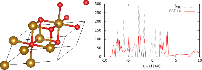
Plot the up and dn spin density of states with energy relative to the Fermi level, following the previous tutorial. Note that both spin channels now have the same density of states profile because there are equal number of up and dn spins per unit cell. As an exercise, examine the orbital-projected density of states on the two Fe atoms; there should be a difference between the majority and minority spin channels on each atom. Note however, that the density of states at the Fermi level is finite, indicating that the structure is metallic, rather than insulating as expected.

The reason for this discrepancy is self-interaction errors for localized electrons in DFT. The d electrons in particular experience an unphysical Coulomb repulsion with themselves, which increases their energy and in this case, the occupied d bands cross the Fermi level rather than remaining entirely below it, thereby making the material metallic. DFT + U is a simple way to correct this issue by adding an energy correction depending on the occupation of localized states using atomic orbital projections. This however introduces a parameter U that could be calculated using perturbation theory, or calibrated to experimental properties of interest such as band gaps or formation energies. For Fe, a typical value of this parameter is 4.3 eV = 0.158 Hartrees, and we include this in the input file FeO.in by adding the command add-U :

add-U Fe d 0.158

which specifies the correction just for d orbitals of species Fe. Also, update the dump-name to PBE+U.$VAR so as to not replace previous outputs, and run "mpirun -n 4 jdftx -i FeO.in | tee PBE+U.out". Note that the magentic moments are larger after adding U because it makes it more favorable for electrons to occupy the high-spin localized orbitals. Additionally, plotting the density of states reveals that the U correction indeed opens up a gap (by pushing down occupied d orbitals in energy relative to unoccupied d orbitals), as shown at the top of the page.

Exercise: examine the electronic band structure: is the band gap direct or indirect?