Most density-functional theory calculations are based in non-relativistic quantum mechanics, where spin decouples completely from the spatial degrees of freedom and only enter in the orbital occupations. Far from the atoms, the electron velocities are indeed much smaller than the speed of light and the non-relativistic approximation is valid. This is however no longer true close to the nuclei for electrons with non-zero angular momentum. Importantly, even valence electrons (with l > 0) in heavy atoms pick up relativsitic effects - especially spin-orbit coupling - from the regions of space close to the nuclei. This tutorial demonstrates the effect of spin-orbit coupling on the band structure of metallic platinum.

In plane-wave calculations using pseudopotentials, these relativistic effects can be built into the pseudopotentials. The GBRV pseudopotentials we have used so far do not have relativistic versions available, so we will use another pseudopotential from the Quantum Espresso pseudopotential library. Download this relativistic pseudopotential, and also this conventional non-relativistic pseudopotential, into your current working directory. We will use a different non-relativistic pseudopotential as well to compare with and identify the relativistic effects, and for this we will use the downloaded one instead of GBRV because its generation parameters are much closer to the relativistic one and we will see less discrepancies simply due to pseudopotential differences.

You should now have two UPF pseudopotential files in your current directory:

Pt.rel-pbe-n-rrkjus_psl.0.1.UPF   #the relativistic one
Pt.pbe-n-rrkjus_psl.0.1.UPF       #the non-relativistic one

Let's start with a non-relativistic band-structure calculation of platinum, exactly as in in the Metals tutorial, but with the new pseudopotential:

#Save the following to common.in:
lattice face-centered Cubic 7.41
ion-species Pt.pbe-n-rrkjus_psl.0.1.UPF
elec-cutoff 20 200    #Above UPF suggests higher charge-density cutoff than GBRV
ion Pt  0 0 0  0

#Save the following to totalE.in:
include common.in
dump End ElecDensity
dump-name totalE.$VAR
kpoint-folding 12 12 12
elec-smearing Fermi 0.01
electronic-SCF

#Save the following to bandstruct.in
include common.in
include bandstruct.kpoints
fix-electron-density totalE.$VAR
elec-n-bands 9
dump End BandEigs
dump-name bandstruct.$VAR

Use the bandstructKpoints script to generate a k-point path and plot script as described in the Band structure calculations tutorial, and run the total energy and band structure calculations using:

mpirun -n 4 jdftx -i totalE.in |  tee totalE.out
mpirun -n 4 jdftx -i bandstruct.in |  tee bandstruct.out

Edit the plot script to reference energies relative to the Fermi level and in eV, and you should get a band structure very similar to the one in the Metals tutorial, with only minor differences due to the pseudopotential.

Now to perform the relativistic (spin-orbit) calculations, similarly make three input files, with the important differences annotated:

#Save the following to common-rel.in:
lattice face-centered Cubic 7.41
ion-species Pt.rel-pbe-n-rrkjus_psl.0.1.UPF   #Different pseudopotential file
elec-cutoff 20 200
ion Pt  0 0 0  0
spintype spin-orbit                           #Relativistic spin type

#Save the following to totalE-rel.in:
include common-rel.in
dump End ElecDensity
dump-name totalE-rel.$VAR
kpoint-folding 12 12 12
elec-smearing Fermi 0.01
electronic-SCF

#Save the following to bandstruct-rel.in
include common-rel.in
include bandstruct.kpoints
fix-electron-density totalE-rel.$VAR
elec-n-bands 18                               #Spinorial: twice as many bands
dump End BandEigs
dump-name bandstruct-rel.$VAR

and run the calculations using:

mpirun -n 4 jdftx -i totalE-rel.in |  tee totalE-rel.out
mpirun -n 4 jdftx -i bandstruct-rel.in |  tee bandstruct-rel.out

Compare the relativistic and non-relativistic output files. The most important difference is that the number of bands is double in the relativistic calculation since the spin degrees of freedom must now be treated explicitly. Additionally, the code also needs to store two spinor components for each wave-function, which along with the band doubling, makes the net memory usage about four times as large as the corresponding non-relativistic calculation. The time taken for the calculations also increases by a similar factor.

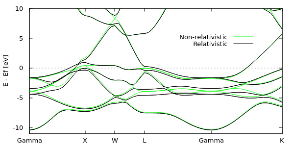
Edit the previous bandstructure plot script to overlay bandstruct-rel.eigenvals, and obtain the plot shown below and at the top of this page. (Hint: you will need to duplicate and edit the nCols and formatString lines in bandstruct.plot.) Notice that the lowest band is unaffected by spin-orbit coupling: this is because this band is dominated by s character (l = 0) and hence has negligible orbital angular momentum. Strong splittings close to 1 eV are observable near the Gamma and L points approximately 4 eV below the Fermi level, and near the X point close to the Fermi level. Spin-orbit coupling usually does not significantly impact geometries and reaction energies, but has a very strong influence on optical properties of materials with heavy elements, because these properties depend directly on energy level spacings.

With this, we have explored three of the four options in spintype. For non-relativistic calculations, no-spin and z-spin correspond to spin-unpolarized and spin-polarized calculations respectively. Analgously, spin-orbit specifies unpolarized relativistic calculations whereas the fourth mode, vector-spin, specifies polarized relativistic calculations. The number of bands and k-vectors will be identical between spin-orbit and vector-spin calculations since all the spin degrees of freedom are treated explicitly anyway. Additionally, in vector-spin mode, you can specify initial-magnetic-moments to initialize the magnetizations on each atom, which are now all vectors with directions (and not just + / - as in z-spin mode). Correspondingly, all magnetization output in the code, such as in the FillingsUpdate lines and in the Lowdin analysis, report a vector direction in addition to magnitude.

Exercise: reproduce the previous tutorial with spins along the x-axis and then again with spins along the y-axis using vector-spin spintype. Note that you can continue to use the non-relativistic GBRV pseudopotentials for this exercise, and you should then get the same answers irrespective of overall spin axis direction (since spin and spatial motion are decoupled).