The previous tutorials calculated properties of neutral surfaces in vacuum and solution. With continuum solvation models of electrolytes (solvent + ions), we can straightforwardly also treat charged surfaces in solution. This is particularly important for electrochemical systems, where the electrode surface is in electrical contact with an external circuit which sets the electron chemical potential (mu). The number of electrons equilibrates to the applied mu and will result in a charged surface, except for the special case when mu is the potential of zero charge (PZC).

The most basic charged surface calculation is identical to the previous tutorials, except for an elec-initial-charge command that sets up a non-zero charge state. This tutorial will instead demonstrate fixed-potential calculations using the target-mu command, which directly sets the electron chemical potential and lets the electron number equilibrate, exactly as in electrochemical systems. Specifically, we will calculate the charge vs potential curve of the Pt(111) surface.

We can collect most of the commands including fluid into the common setup file:

#Save the following to common.in:
lattice Hexagonal 5.23966 36
ion Pt  0.333333 -0.333333 -0.237676   1
ion Pt -0.333333  0.333333 -0.118838   1
ion Pt  0.000000  0.000000  0.000000   1
ion Pt  0.333333 -0.333333  0.118838   1
ion Pt -0.333333  0.333333  0.237676   1

ion-species GBRV/$ID_pbesol.uspp
elec-ex-corr gga-PBEsol
elec-cutoff 20 100

coulomb-interaction Slab 001
coulomb-truncation-embed 0 0 0

kpoint-folding 12 12 1
elec-smearing Fermi 0.01

fluid LinearPCM
pcm-variant CANDLE
fluid-solvent H2O
fluid-cation Na+ 1.
fluid-anion F- 1.

dump-name common.$VAR      #This will overwrite outputs from successive runs
initial-state common.$VAR  #This will initialize from the preceding calculation
dump End State BoundCharge

Note that we have included the geometry here instead of in ionpos/lattice files since we plan to skip geometry optimization for expediency in this tutorial too.

Start with a neutral calculation (in non-adsorbing aqueous NaF electrolyte):

#Save the following to Neutral.in
include common.in
electronic-SCF

which we run as:

jdftx -i Neutral.in | tee Neutral.out

Next, we setup the fixed potential calculations using the input file:

#Save the following to Charged.in:
include common.in
electronic-minimize nIterations 200
target-mu ${mu}

Note that we have used the robust, but slower, minimization algorithm instead of SCF because the SCF algorithm does not reliably converge in fixed-potential mode (yet) due to a charge-sloshing instability between the system and the electron reservoir.

We will now run a sequence of fixed-potential calculations for mu varying from -1 to +1 eV relative to the neutral potential (PZC) of -0.2015 Hartrees (final mu from Neutral.out).

#!/bin/bash
for iMu in {-10..10}; do
    export mu="$(echo $iMu | awk '{printf("%.4f", -0.2015+0.1*$1/27.2114)}')"
    mpirun -n 4 jdftx -i Charged.in | tee Charged$mu.out
    mv common.nbound Charged$mu.nbound
done

Save the above to run.sh, , give execute permissions using "chmod +x run.sh", and execute using "./run.sh". This will take a while (~ 1 hour on a laptop)! Note that the first line within the for loop calculates the current mu value, and the last line moves the bound charge output before it is overwritten by the next run. Also note that the first calculation takes the longest because it needs to move from the neutral state by 1 eV to the end of the range. The intermediate calculations are quicker since they only shift the potential by 0.1 eV, and each calculation starts at the final state of the previous one (all stored in common.$VAR).

Examine one of the output files, say Charged-0.2382.out. Notice that the energy output is now called G, instead of F. This is the grand free energy, G = F - mu N, where N is the number of electrons (also check the energy components output at the end). G is the appropriate free energy that satisfies a variational theorem at fixed electron chemical potential and temperature, and no longer F, which was the appropriate free energy at fixed electron number and temperature. (Recall the discussion of F vs Etot in the Metals tutorial.)

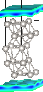
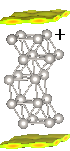
Next examine the bound charge distribution in the fluid for the two extremes of potential using:

createXSF Charged-0.2382.out Charged-0.2382.xsf Charged-0.2382.nbound
createXSF Charged-0.1648.out Charged-0.1648.xsf Charged-0.1648.nbound

We need to specify the full file name for the bound charge file, rather than just the suffix 'nbound', because we moved the file in our run script. Visualizing these XSF files in VESTA, you shoud see distributions as shown at the top of this page. Note that the bound charge density is closer and larger next to the negatively charged surface as compared to the positively charged one due to the charge-asymmetry of CANDLE, exactly as we saw before in the Solvation of ions tutorial.

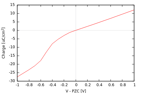
Finally, we will extract the charging curve of the Pt(111) surface:

#!/bin/bash
for file in Charged*.out; do
    awk '/FillingsUpdate/ {mu=$3; N=$5} END {print mu, N}' "$file"
done

Save the above to collectResults.sh, give execute permissions using "chmod +x collectResults.sh", and execute using "./collectResults.sh | tee mu_N.dat". Note that the above script uses awk to extract the final mu and nElectrons from each calculation. We can plot the extracted results using gnuplot:

#Within an interactive gnuplot session:
A = 2*((5.23966*0.529e-8)**2)*sin(pi/3) #top+bottom surface area in cm^2
qe = -1.602e-13                         #electron charge in microCoulombs
mu0 = -0.2015                           #mu corresponding to PZC
N0 = 80                                 #Nelectrons in neutral surface
set xlabel "V - PZC [V]"
set ylabel "Charge [uC/cm^2]"
set xzeroaxis
set yzeroaxis
unset key
plot "mu_N.dat" u ((mu0-$1)*27.2114):(($2-N0)*qe/A) w l

We have switched units and sign conventions to those commonly used in electrochemistry. The resulting plot is shown at the top of this page: note the change in slope and magnitude of charge density upon crossing the neutral potential, again a result of the charge asymmetry in CANDLE. The average slopes correspond to a capacitance of roughly 10 uF/cm² on the positive side and 25 uF/cm² on the negative side.

Exercise: calculate and plot the derivative dN/dmu as a function of potential using a finite difference formula. This gives you the differential capacitance.