Silicon, the crystalline solid we have worked with is a semiconductor with a band gap which we identified in the tutorials on Band structure calculations and Density of states. This gap clearly demarcates occupied states from unoccupied states for all k-points, so electron 'fillings' are straightforward: the lowest (nElectrons/2) bands of all k-points are filled, and the remaining are empty. This is no longer true for metals, where one or more bands are partially filled, and these fillings (or occupation factors) must be optimized self-consistently. This tutorial introduces such a calculation for platinum.

Platinum is a face-centered cubic metal with a cubic lattice constant of 3.92 Angstroms (7.41 bohrs), which we can specify easily in the input files:

#Save the following to common.in:
lattice face-centered Cubic 7.41
ion-species GBRV/$ID_pbesol.uspp
elec-ex-corr gga-PBEsol
elec-cutoff 20 100
ion Pt  0 0 0  0      #Single atom per unit cell

and

#Save the following to totalE.in:
include common.in
dump End ElecDensity State
dump-name totalE.$VAR
kpoint-folding 12 12 12     #Metals need more k-points
elec-smearing Fermi 0.01  #Set fillings using Fermi function at T = 0.01 Hartrees
electronic-SCF

The only new command is elec-smearing which specifies that the fillings must be set using a Fermi function based on the current Kohn-Sham eigenvalues, rather than determined once at startup (the default we implicitly used so far). The first parameter of this command specifies the functional form for the occupations, in this case selecting a Fermi function (see elec-smearing for other options). The second parameter determines the width in energy over which the Fermi function goes from one to zero (occupied to unoccupied).

Metals are much more sensitive to k-point sampling, because for some bands, a part of the Brillouin zone is filled and the remainder is empty, separated by a Fermi surface. The number of k-points directly determines how accurately the Fermi surface(s) can be resolved. The Fermi temperature is essentially a smoothing parameter that allows us to resolve the Fermi surface accurately at moderate k-point counts. Note that the tempreature we chose is around ten times room temperature in order to increase the smoothing and use a practical number of k-points.

Finally, we have selected the PBEsol exchange-correlation functional using the elec-ex-corr command, which is generally more accurate than PBE for solids (especially for metals). Correspondingly, we selected PBEsol pseudopotentials from the GBRV set.

Run the calculation above as usual using

mpirun -n 4 jdftx -i totalE.in | tee totalE.out

and examine the output file. The main difference is that every SCF line is preceded by a line starting with FillingsUpdate. This line reports the chemical potential, mu, of the Fermi function that produces the correct number of electrons with the current Kohn-Sham eigenvalues, and the number of electrons, nElectrons, which of course stays constant.

Also notice that the energy in the SCF lines is called F instead of Etot. The total energy Etot satisfies a variational theorem at fixed occupations, which we dealt with so far. However, now the occupations equilibrate at a specified temperature T, and the Helmholtz free energy F = E - TS, where S is the electronic entropy, is the appropriate variational free energy to work with. Note the corresponding changes in the energy component printout at the end as well.

Additionally, in the initialization, note that nBands is now larger than nElectrons/2, since the code needs a few empty states to use Fermi fillings. At the end of the calculation, when dumping State, note that the calculation now outputs files with suffix wfns, fillings and Haux. The wfns contain the wavefunctions (Kohn-Sham orbitals) as before, while fillings contains the occupations and Haux contains auxiliary Hamiltonian matrices used by the minimize algorithm with Fermi fillings. When running calculations with Fermi fillings, initial-state will try to read in all these files instead of wfns alone.

Examine the fillings file using:

binaryToText totalE.fillings 12

The last parameter 12 equals the number of bands, and this causes binaryToText to display the result as a matrix with 12 columns. In this case, the rows then correspond to the reduced k-point (there will be 72 of them). Notice that the first five columns (bands) are approximately 2 (including spin factor) throughout, and columns ten onwards are approximately 0 throughout, whereas columns six through nine have empty, partially occupied and occupied states implying that they cross the Fermi level.

We can also see this in the band structure. Generate bandstruct.kpoints as shown in the Band structure calculations tutorial, create an input file:

#Save the following to bandstruct.in
include common.in
include bandstruct.kpoints
fix-electron-density totalE.$VAR
elec-n-bands 12
dump End BandEigs
dump-name bandstruct.$VAR

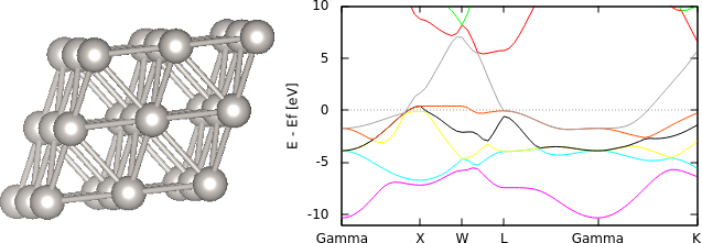
and run "mpirun -n 4 jdftx -i bandstruct.in". Note that the band structure input file is almost identical to the Si band structure tutorial, varying only in the number of bands. (The band structure calculation should not specify Fermi fillings.) Edit bandstruct.plot to reference the energies relative to mu (from the final FillingsUpdate line, or equivalently using dump End EigStats). and convert to eV (see the end of the Band structure calculations tutorial). Also update the y-axis range to exclude energies far below the Fermi level (mu), which we have set to zero in the plot and annotated with a dotted line. (Try it without doing so; the three bands you will see far below the Fermi level are inner shell 5p electrons of the platinum which have been treated as valence electrons in the GBRV Pt pseudopotential, which you can check in the pseudopotential section of the initialization log.) Run bandstruct.plot to get the bandstructure shown above. Notice that bands number six - nine from the bottom cross the Fermi level (mu), remembering that three of them are below the bottom margin.

Finally, as an exercise, study the k-point convergence of this metal calculation following the outline of the Brillouin-zone sampling tutorial. How does the k-point convergence of the energy compare to the Silicon case? Try reducing the temperature in elec-fermi-filings from 0.01 to 0.005 and redo the k-point convergence study. Compare the k-point covergence between the two temperatures. Analytically, you expect the number of k-points per dimension to be inversely proportional to the Fermi temperature (smoothing width) in order to keep the accuracy (relative to the true infinite k-points limit) constant.