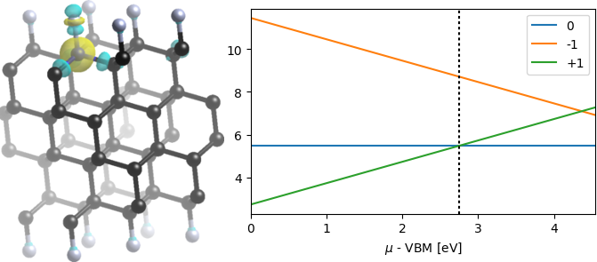
We now deal with localized point defects at or near the surface of a 3D material, which largely follows the procedure of a point defect in the bulk (interior) of a 3D material shown in the previous tutorial, with a few extra steps. In particular, we will consider the same N_C (nitrogen substituting carbon) point defect as the previous tutorial, but at the (111) surface of diamond instead of the bulk.

Surface unit cell

First construct a (111) surface unit cell of diamond with four layers. This is very similar to the Pt(111) setup, except with two C atoms within the FCC primitive cell (instead of a single Pt atom). However, we will additionally need to terminate the dangling bonds at the surface. This is particularly important for covalent-bonded materials and semiconductors/insulators compared to metals, because the dangling bonds may introduce surface states within the bulk band gap which will interfere with our calculation of defect states. H-termination is standard for dangling C bonds in organic chemistry, but interestingly H-terminated diamond has a negative electron affinity that will make calculating -1 charge states of surface defects unstable. Let us consider an F-terminated diamond (111) surface instead, which is structurally as simple as H-termination and exhibits a positive electron affinity:

#Save the following to surface.in
lattice Hexagonal 4.766 30
coulomb-interaction Slab 001
coulomb-truncation-embed 0 0 0

ion F 0.333333 0.666667 -0.297367 1
ion C 0.333333 0.666667 -0.210755 1
ion C 0.666667 0.333333 -0.178332 1
ion C 0.666667 0.333333 -0.081060 1
ion C 0.000000 0.000000 -0.048636 1
ion C 0.000000 0.000000  0.048636 1
ion C 0.333333 0.666667  0.081060 1
ion C 0.333333 0.666667  0.178332 1
ion C 0.666667 0.333333  0.210755 1
ion F 0.666667 0.333333  0.297367 1

ion-species GBRV/$ID_pbe.uspp
elec-cutoff 20 100

kpoint-folding 4 4 1
elec-smearing Fermi 0.01

electronic-SCF
dump End None

We do not need any information from this surface unit cell that we won't also get from the perfect supercell below, so we can skip running jdftx on surface.in. Instead, we need to determine the spatial profile of dielectric response for the charged defect correction. To do this, we will first apply a small electric field normal to the slab in one direction:

#Save the following to minus.in
include surface.in

electric-field 0 0 -0.001
dump End Dtot

Run jdftx on minus.in to get the electrostatic potential for a small field along the -z direction. We will then apply a field along the +z direction of the same magnitude:

#Save the following to plus.in
include surface.in

electric-field 0 0 +0.001
slab-epsilon minus.d_tot 2.  0 0 -0.001

Run jdftx on plus.in to get the dielectric profile computed by a finite difference with respect to the reference electrostatic potential in minus.d_tot (see command slab-epsilon). The resulting dielectric profile in plus.slabEpsilon is shown below, with the surface structure overlaid for reference:

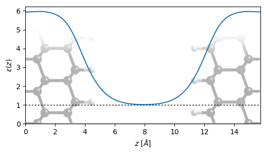
Note that the dielectric function varies smoothly from 1 in the vacuum region to approximately 5.9 in the center of the slab, which agrees very well with the experimental dielectric constant of 5.8 used in the previous tutorial. Since we did not optimize the ionic positions, this corresponds to \( \epsilon_\infty \), and we will consistently not do ionic optimizations below. As discussed in Defects in 3D materials, if we perform ionic optimization of the defect structure, we should use \( \epsilon_0 \) instead, which can be optimized exactly as above with ionic-minimize added to both minus.in and plus.in.

Finally, note that the second argument of slab-epsilon is a Gaussian smoothing which should be adjusted to the smallest value that does not show an oscillating profile within the material. We have set the value above to roughly half the spacing between atomic layers in diamond (111) which is sufficient to damp out the oscillations.

Exercise: Run plus.in with smaller and larger values of the Gaussian smoothing to check the impact on the dielectric profile.

Surface supercell

Next, exactly as in the bulk defect case, we need to construct a supercell so that we separate the defect from its periodic images. The slab already breaks periodicity along the z direction, so we now need to repeat the unit cell only along the two remaining directions. For computational expediency, we work here with a 2x2x1 supercell by expanding the first two lattice vectors by a factor of 2 and then halving, repeating and offsetting the first two fractional coordinates:

#Save the following to supercell.in
lattice Hexagonal 4.766 30
latt-scale 2 2 1
coulomb-interaction Slab 001
coulomb-truncation-embed 0 0 0

ion F 0.166667 0.333333 -0.297367 1
ion C 0.166667 0.333333 -0.210755 1
ion C 0.333333 0.166667 -0.178332 1
ion C 0.333333 0.166667 -0.081060 1
ion C 0.000000 0.000000 -0.048636 1
ion C 0.000000 0.000000  0.048636 1
ion C 0.166667 0.333333  0.081060 1
ion C 0.166667 0.333333  0.178332 1
ion C 0.333333 0.166667  0.210755 1
ion F 0.333333 0.166667  0.297367 1

ion F 0.166667 0.833333 -0.297367 1
ion C 0.166667 0.833333 -0.210755 1
ion C 0.333333 0.666667 -0.178332 1
ion C 0.333333 0.666667 -0.081060 1
ion C 0.000000 0.500000 -0.048636 1
ion C 0.000000 0.500000  0.048636 1
ion C 0.166667 0.833333  0.081060 1
ion C 0.166667 0.833333  0.178332 1
ion C 0.333333 0.666667  0.210755 1
ion F 0.333333 0.666667  0.297367 1

ion F 0.666667 0.333333 -0.297367 1
ion C 0.666667 0.333333 -0.210755 1
ion C 0.833333 0.166667 -0.178332 1
ion C 0.833333 0.166667 -0.081060 1
ion C 0.500000 0.000000 -0.048636 1
ion C 0.500000 0.000000  0.048636 1
ion C 0.666667 0.333333  0.081060 1
ion C 0.666667 0.333333  0.178332 1
ion C 0.833333 0.166667  0.210755 1
ion F 0.833333 0.166667  0.297367 1

ion F 0.666667 0.833333 -0.297367 1
ion C 0.666667 0.833333 -0.210755 1
ion C 0.833333 0.666667 -0.178332 1
ion C 0.833333 0.666667 -0.081060 1
ion C 0.500000 0.500000 -0.048636 1
ion C 0.500000 0.500000  0.048636 1
ion C 0.666667 0.833333  0.081060 1
ion C 0.666667 0.833333  0.178332 1
ion C 0.833333 0.666667  0.210755 1
ion F 0.833333 0.666667  0.297367 1

ion-species GBRV/$ID_pbe.uspp
elec-cutoff 20 100

kpoint-folding 2 2 1
elec-smearing Fermi 0.01

electronic-SCF
converge-empty-states yes
dump End EigStats ElecDensity Dtot

Run jdftx on supercell.in: note that it has nStates (reduced k-points) = 2, so if you are running it with MPI on a four core system, you should use "mpirun -n 2 jdftx -c2 -i supercell.in". On a compute cluster, you can use up to two nodes with "mpirun -n 2 jdftx -cX -i supercell.in", where X is the number of cores per node. See Getting started for further details.

This calculation outputs the eigenvalue statistics, electron density and electrostatic potential. Note that the HOMO and LUMO levels are overall offset from the bulk: they are now on an absolute scale referenced to zero outside the surface, and correspond to the ionization potential and electron affinity respectively of F-terminated diamond.

Neutral defect

We can now introduce a neutral defect by substituting a surface carbon atom with nitrogen:

#Save the following to N_C-0.in:
lattice Hexagonal 4.766 30
latt-scale 2 2 1
coulomb-interaction Slab 001
coulomb-truncation-embed 0 0 0

ion F 0.166667 0.333333 -0.297367 1
ion C 0.166667 0.333333 -0.210755 1
ion C 0.333333 0.166667 -0.178332 1
ion C 0.333333 0.166667 -0.081060 1
ion C 0.000000 0.000000 -0.048636 1
ion C 0.000000 0.000000  0.048636 1
ion C 0.166667 0.333333  0.081060 1
ion C 0.166667 0.333333  0.178332 1
ion N 0.333333 0.166667  0.210755 1  #Note C replaced by N
ion F 0.333333 0.166667  0.297367 1

ion F 0.166667 0.833333 -0.297367 1
ion C 0.166667 0.833333 -0.210755 1
ion C 0.333333 0.666667 -0.178332 1
ion C 0.333333 0.666667 -0.081060 1
ion C 0.000000 0.500000 -0.048636 1
ion C 0.000000 0.500000  0.048636 1
ion C 0.166667 0.833333  0.081060 1
ion C 0.166667 0.833333  0.178332 1
ion C 0.333333 0.666667  0.210755 1
ion F 0.333333 0.666667  0.297367 1

ion F 0.666667 0.333333 -0.297367 1
ion C 0.666667 0.333333 -0.210755 1
ion C 0.833333 0.166667 -0.178332 1
ion C 0.833333 0.166667 -0.081060 1
ion C 0.500000 0.000000 -0.048636 1
ion C 0.500000 0.000000  0.048636 1
ion C 0.666667 0.333333  0.081060 1
ion C 0.666667 0.333333  0.178332 1
ion C 0.833333 0.166667  0.210755 1
ion F 0.833333 0.166667  0.297367 1

ion F 0.666667 0.833333 -0.297367 1
ion C 0.666667 0.833333 -0.210755 1
ion C 0.833333 0.666667 -0.178332 1
ion C 0.833333 0.666667 -0.081060 1
ion C 0.500000 0.500000 -0.048636 1
ion C 0.500000 0.500000  0.048636 1
ion C 0.666667 0.833333  0.081060 1
ion C 0.666667 0.833333  0.178332 1
ion C 0.833333 0.666667  0.210755 1
ion F 0.833333 0.666667  0.297367 1

ion-species GBRV/$ID_pbe.uspp
elec-cutoff 20 100

kpoint-folding 2 2 1
elec-smearing Fermi 0.01

electronic-SCF
dump End Dtot ElecDensity

For the neutral defect, we can calculate the formation energy by comparing to the energy of the perfect supercell, with reference energies (chemical potentials) for C and N set by bulk diamond and N₂ respectively, exactly as discussed in Defects in 3D materials. This results in a neutral formation energy of approximately 5.5 eV, which is larger than that of the bulk defect. This indicates that the N-F bond is weaker than the C-F bond by a greater amount than the N-C bond is weaker than the C-C bond for the bulk case.

Exercise: Compute the neutral formation energies for N_C defects positioned deeper within the slab. How does the formation energy compare with the bulk case for a defect in the center of the slab?

Charged defects

The procedure for charged defects at the surface is very similar to the bulk case, with the only difference being that charged-defect-correction expects a dielectric profile computed by slab-epsilon as we did above instead of a single number. (See [33] for implementation details.) Run jdftx on N_C-1.in for the -1 charge state:

#Save the following to N_C-1.in
include N_C-0.in

elec-initial-charge +1                             #One extra electron
charged-defect 0.333333 0.166667 0.210755  +1  1   #Gaussian charge model
charged-defect-correction \
    supercell.d_tot  \  #reference potential for alignment
    plus.slabEpsilon \  #slab dielectric profile
    5.               \  #cutoff distance for alignment potential
    1.                  #smoothness in alignment potential cutoff

and on N_C+1.in for the +1 charge state:

#Save the following to N_C+1.in
include N_C-0.in

elec-initial-charge -1                             #One less electron
charged-defect 0.333333 0.166667 0.210755  -1  1   #Gaussian charge model
charged-defect-correction \
    supercell.d_tot  \  #reference potential for alignment
    plus.slabEpsilon \  #slab dielectric profile
    5.               \  #cutoff distance for alignment potential
    1.                  #smoothness in alignment potential cutoff

Collect the energies from each of these calculations into the analysis script from the Defects in 3D materials tutorial:

import numpy as np
import matplotlib.pyplot as plt

#Bulk properties:
muC = -11.408263/2 #energy per carbon atom in bulk
muN = -19.962539/2 #energy per N atom in N2 molecule
HOMO = -0.289210
LUMO = -0.122029

#Supercell properties:
Esup  = -376.910492 #energy of perfect supercell
EN_C0 = -380.986456 #energy of neutral N_C defect
EN_CM = -381.617332+0.561685 #energy of -1 N_C defect (including correction)
EN_CP = -381.169310+0.371130 #energy of +1 N_C defect (including correction)

#Compute defect formation energies:
# ... 
# ...

Note that the bottom part of the script is identical to the previous case and has not been repeated. We have only replaced the supercell energies (and corrections where applicable), in addition to the HOMO and LUMO levels. The result is a charge transition level (CTL) for -1|0 of 6.0 eV wrt VBM, corresponding to an acceptor level with ionization energy 6.0 eV. The CTL for 0|+1 is 2.7 eV wrt VBM corresponding to a donor level with an ionization energy 1.8 eV (below CBM). Thus the surface N_C defect has a higher formation energy, deeper acceptor level and slightly shallower donor level than the bulk N_C defect.

Exercise: converge the charged defect results with supercell size. Plot the results as a function of supercell size with and without the correction. How big of a supercell would you need for 0.1 eV accuracy with and without the correction?

Exercise: test the effect of surface termination on the defect properties, perhaps including -H and -OH terminated diamond (111). Also study the property of these defects at other surface orientations eg. (100).